5.2. Acoustic Peaks and the Cosmological Parameters

The early universe was a plasma of photons and baryons and can be treated as a single fluid. [24] Baryons fell into the gravitational potential wells created by the density fluctuations and were compressed. This compression gave rise to a hotter plasma thus increasing the outward radiation pressure from the photons. Eventually, this radiation pressure halted the compression and caused the plasma to expand (rarefy) and cool producing less radiation pressure. With a decreased radiation pressure, the region reached the point where gravity again dominated and produced another compression phase. Thus, the struggle between gravity and radiation pressure set up longitudinal (acoustic) oscillations in the photon-baryon fluid. When matter and radiation decoupled at recombination the pattern of acoustic oscillations became frozen into the CMB. Today, we detect the evidence of the sound waves (regions of higher and lower density) via the primary CMB anisotropies.

It is well known that any sound wave, no matter how complicated, can be decomposed into a superposition of wave modes of different wavenumbers k, each k being inversely proportional to the physical size of the corresponding wave (its wavelength), k 1/. Observationally, what is seen is a projection of the sound waves onto the sky. So, the wavelength of a particular mode is observed to subtend a particular angle on the sky. Therefore, to facilitate comparison between theory and observation, instead of a Fourier decomposition of the acoustic oscillations in terms of sines and cosines, we use an angular decomposition (multipole expansion) in terms of Legendre polynomials P(cos). The order of the polynomial (related to the multipole moments) plays a similar role for the angular decomposition as the wavenumber k does for the Fourier decomposition. For 2 the Legendre polynomials on the interval [-1,1] are oscillating functions containing a greater number of oscillations as increases. Therefore, the value of is inversely proportional to the characteristic angular size of the wave mode it describes

(44)

Experimentally, temperature fluctuations can be analyzed in pairs, in directions and ' that are separated by an angle so that ^. ' = cos. By averaging over all such pairs, under the assumption that the fluctuations are Gaussian, we obtain the two-point correlation function, C(), which is written in terms of the multipole expansion

(45)

the C coefficients are called the multipole moments.

As predicted, analysis of the temperature fluctuations does in fact reveal patterns corresponding to a harmonic series of longitudinal oscillations. The various modes correspond to the number of oscillations completed before recombination. The longest wavelength mode, subtending the largest angular size for the primary anisotropies, is the fundamental mode - this was the first mode detected. There is now strong evidence that both the 2^nd and 3^rd modes have also been observed. [20] - [22]

The distance sound waves could have traveled in the time before recombination is called the sound horizon, r_s. The sound horizon is a fixed physical scale at the surface of last scattering. The size of the sound horizon depends on the values of cosmological parameters. The distance to the surface of last scattering, d_sls, also depends on cosmological parameters. Together, they determine the angular size of the sound horizon (see Fig. 3)

(46)

in the same way that the angle subtended by the planet Jupiter depends on both its size and distance from us. Analysis of the temperature anisotropies in the CMB determine and the cosmological parameters can be varied in r_s and d_sls to determine the best-fit results.

We can estimate the sound horizon by the distance that sound can travel from the big bang, t = 0, to recombination t_*

(47)

where z_* is the redshift parameter at recombination (z_* 1100) [25], _r is the density parameter for radiation (photons), c_s is the speed of sound in the photon-baryon fluid, given by [26]

(48)

which depends on the baryon-to-photon density ratio, and dt is determined by an expression similar to Eq. (36), except at an epoch in which radiation plays a more important role. The energy density of radiation scales as [27] _r a^-4, so with the addition of radiation, Eq. (33) generalizes to

(49)

which, upon using Eq. (35) and _r + _m + + _k = 1, leads to

(50)

The distance to the surface of last scattering, corresponding to its angular size, is given by what is called the angular diameter distance. It has a simple relationship to the luminosity distance [15] d given in Eq. (37)

(51)

The location of the first acoustic peak is given by d_sls / r_s and is most sensitive to the curvature of the universe _k.

To get a feeling for this result, we can consider a very simplified, heuristic calculation. We will consider a prediction for the first acoustic peak for the case of a flat universe. To leading order, the speed of sound in the photon-baryon fluid, Eq. (48), is constant c_s = c / 3^1/2. We further make the simplifying assumption that the early universe was matter-dominated (there is good reason to believe that it was which will be discussed in the next section). With these assumptions, Eqs. (49) and (47) yield (dropping the '0' from the density parameters)

(52)

which gives

(53)

The distance to the surface of last scattering, in our flat universe model, will depend on both _m and . Following a procedure similar to that which lead to Eq. (37), the radial coordinate of the surface of last scattering, r_sls (not to be confused with r_s), is determined by

(54)

which does not yield a simple result. Using a binomial expansion, the integrand can be approximated as _m^-1/2(1 + z)^-3/2 - ( / 2_m^3/2)(1 + z)^-9/2 and the integral is more easily handled. The distance is then determined by d_sls = r_sls / (1 + z_*) which gives

(55)

Using = 1 - _m and neglecting the higher order terms then gives

(56)

Combining Eqs. (53) and (56) to get our prediction for the first acoustic peak gives

(57)

This result is consistent with the more detailed result that [28]

(58)

where, in our calculation _k = 0. Equation (58) suggests that a measurement of 200 implies a flat universe. The BOOMERanG [21] collaboration found 197±6, and the MAXIMA-1 [20] collaboration measured 220. Additional simplified illustrations for how the cosmological parameters can be obtained from the acoustic peak can be found in Ref. 29.

Experimental results, such as those quoted above, are determined by plotting the power spectrum (power per logarithmic interval), ( T)², given by

(59)

or by the square root of this quantity. The power spectrum may be quickly calculated for a given cosmological model using a code such as CMBFAST which is freely available online. [30] The solid curve in Fig. 4 was calculated using CMBFAST and the data points are only a representative few included to show the kind of agreement between theory and experiment that exists.

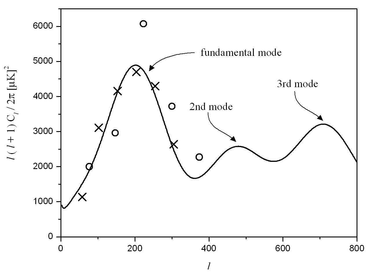Figure 4. The power spectrum. The solid curve is a theoretical power spectrum calculated using CMBFAST. [30] The open circles are from Ref. 20 and the crosses are from Ref. 21. Notice that the first peak corresponding to the fundamental acoustic mode occurs near = 200, signifying a flat universe.

While the location of the first acoustic peak helps to fix _k, other features of the power spectrum help to determine the baryon density. Since baryons are the primary cause of the gravitational potential wells that help generate the acoustic oscillations, they affect the power spectrum in several ways. The relative heights of the peaks are an indication of _b in that an increase in baryon density results in an enhancement of the odd peaks. An increase in baryon density also leads to enhanced damping at higher multipoles. [31]

It is important to recognize that the constraints on cosmological parameters obtained through this sort of analysis are correlated so that the range of possible values of , for example, depends on what is assumed for the possible range of values of the Hubble constant. Therefore, it is customary to incorporate results from other observational (or theoretical) work in the analysis of the CMB data. With this in mind, we use the value of the Hubble constant stated in Eq. (30). Given this assumption, a combined study of the CMB anisotropy data from the BOOMERanG [22], MAXIMA-1 [21], and COBE-DMR [32] collaborations suggests the following values for the two cosmological parameters being considered here [33]:

(60)

As with the type Ia supernova results, the best-fit CMB results predict an essentially flat universe. In fact, it is quite possible to adopt a model with _k 0 and still obtain a very good fit to the data along with reasonable values for the other cosmological parameters. [33] Again, the CMB data also provides values for additional cosmological parameters, but the curvature and baryon densities are perhaps the most accurately constrained at this time.

Even though the recent revolution in cosmology was ignited by the type Ia supernova and CMB anisotropy results, it is also important to acknowledge prior work toward constraining the cosmological parameters. This work includes investigations on gravitational lensing [34], large-scale structure [35], and the ages of stars, galaxies, and globular clusters [36]. Without this work, the ability to use the supernova and CMB data to place fairly tight restrictions on the major cosmological parameters would be significantly diminished.