6. CMBR AND LSS CONSTRAINTS

The most important source of information on the cosmological parameters are the anisotropies observed in the CMBR temperature and polarization maps over the sky. The temperature angular power spectrum has been measured and analyzed since 1992 [1], whereas the polarization spectrum is very recent [8] and has not yet been analyzed to obtain values for the dynamical parameters. Given the temperature angular power spectrum, the polarization spectrum is predicted with essentially no free parameters. At the moment one can say that the temperature angular power spectrum supports the current model of the Universe as defined by the dynamical parameters obtained from the temperature angular power spectrum.

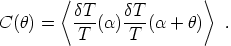
Temperature fluctuations in the CMBR around a mean temperature in a direction on the sky can be analyzed in terms of the autocorrelation function C() which measures the average product of temperatures in two directions separated by an angle ,

(25)

For small angles () the temperature autocorrelation function can be expressed as a sum of Legendre polynomials P() of order , the wave number, with coefficients or powers a²,

(26)

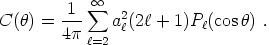
All analyses start with the quadrupole mode = 2 because the = 0 monopole mode is just the mean temperature over the observed part of the sky, and the = 1 mode is the dipole anisotropy due to the motion of Earth relative to the CMBR. In the analysis the powers a² are adjusted to give a best fit of C() to the observed temperature. The resulting distribution of a² values versus is the power spectrum of the fluctuations, see Figure 2. The higher the angular resolution, the more terms of high must be included.

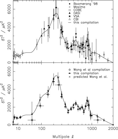Figure 2. Top panel: a compilation of recent CMB data [38]. The solid line shows the result of a maximum-likelihood fit to the power spectrum allowing for calibration and beam uncertainty errors in addition to intrinsic errors. Bottom panel: the solid line is as above, the solid squares [38] and the crosses [41] give the points at which the amplitude of the power spectrum was estimated. For details, see reference [38].

In Section 4 we already noted that the relative magnitudes of the first and second acoustic peaks are sensitive to _b. The position of the first acoustic peak in multipole - space is sensitive to ₀, which makes the CMBR information complementary (and in _m, - space orthogonal) to the supernova information. A decrease in ₀ corresponds to a decrease in curvature and a shift of the power spectrum towards high multipoles. An increase in (in flat space) and a decrease in h (keeping _b h² fixed) both boost the peaks and change their location in - space.

Let us now turn to the distribution of matter in the Universe which can, to some approximation, be described by the hydrodynamics of a viscous, non-static fluid. In such a medium there naturally appear random fluctuations around the mean density (t), manifested by compressions in some regions and rarefactions in other regions. An ordinary fluid is dominated by the material pressure, but in the fluid of our Universe three effects are competing: radiation pressure, gravitational attraction and density dilution due to the Hubble flow. This makes the physics different from ordinary hydrodynamics, regions of overdensity are gravitationally amplified and may, if time permits, grow into large inhomogenities, depleting adjacent regions of underdensity.

Two complementary techniques are available for theoretical modelling of galaxy formation and evolution: numerical simulations and semi-analytic modelling. The strategy in both cases is to calculate how density perturbations emerging from the Big Bang turn into visible galaxies. This requires following through a number of processes: the growth of dark matter halos by accretion and mergers, the dynamics of cooling gas, the transformation of cold gas into stars, the spectrophotometric evolution of the resulting stellar populations, the feedback from star formation and evolution on the properties of prestellar gas, and the build-up of large galaxies by mergers.

As in the case of the CMBR, an arbitrary pattern of fluctuations can be mathematically described by an infinite sum of independent waves, each with its characteristic wavelength or comoving wave number k and its amplitude _k. The sum can be formally expressed as a Fourier expansion for the density contrast at comoving spatial coordinate r and world time t,

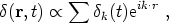(27)

where k is the wave vector.

Analogously to Eq. (23) a density fluctuation can be expressed in terms of the dimensionless mass autocorrelation function

(28)

which measures the correlation between the density contrasts at two points r and r₁. The powers |_k|² define the power spectrum of the rms mass fluctuations,

(29)

Thus the autocorrelation function (r) is the Fourier transform of the power spectrum. This is similar to the situation in the context of CMB anisotropies where the waves represented temperature fluctuations on the surface of the surrounding sky, and the powers a² were coefficients in the Legendre polynomial expansion Eq. (24).

With the lack of more accurate knowledge of the power spectrum one assumes for simplicity that it is specified by a power law

(30)

where n_s is the spectral index of scalar fluctuations. Primordial gravitational fluctuations are expected to have an equal amplitude on all scales. Inflationary models also predict that the power spectrum of matter fluctuations is almost scale-invariant as the fluctuations cross the Hubble radius. This is the Harrison-Zel'dovich spectrum, for which n_s = 1 (n_s = 0 would correspond to white noise).

Since fluctuations in the matter distribution has the same primordial cause as CMBR fluctuations, we can get some general information from CMBR. There, increasing n_s will raise the angular spectrum at large values of with respect to low . Support for 1.0 come from all the available analyses: combining the results of references [38], [41], [43] by the averaging prescription in Section 4, we find

(31)

Phenomenological models of density fluctuations can be specified by the amplitudes _k of the autocorrelation function (r). In particular, if the fluctuations are Gaussian, they are completely specified by the power spectrum P(k). The models can then be compared to the real distribution of galaxies and galaxy clusters, and the phenomenological parameters determined.

As we noted in Section 4, there are several joint compilations of CMBR power spectra and LSS power spectra of which we are interested in the three largest ones [38], [41], [43]. Combining their results for _m by the averaging prescription in Section 4, we find

(32)

If the Universe is spatially flat so that ₀ = 1, this gives immediately the value = 0.71 with slightly better precision than above. To check this assumption we can quote reference [43] from their Table 5 where they use all data,

(33)

Note, however, that this result has been obtained by marginalizing over all other parameters, thus its small statistical errors are conditional on n_s, _m, _b being anything, and we have no prescription for estimating a systematic error.

A value for can be found by adding - _m in Eq. (22) to _m, thus = 0.79 ± 0.12. A better route appears to be to combine Eqs. (30) and (31) to give

(34)

Still a third route is to add ₀ and - _m, or to subtract them, respectively. Then one obtains

The routes making use of - _m from Eq. (22) are, however, making multiple use of the supernova information, so we discard them.

Before ending this Section, we can quote values also for w and q₀. The notation here implies that w is taken as the equation of state of a quintessence component, so that its value could be w > -1. The equation of state of a cosmomological constant component is of course w = -1. In a flat universe w is completely correlated to and therefore also to _m.

We choose to quote the analysis by Bean and Melchiorri [47] who combine CMBR power spectra from COBE-DMR [1], MAXIMA [39], BOOMERANG [40], DASI [6], the supernova data from HSST [10] and SCP [11], the HST Hubble constant [9] quoted in Eq. (15), the baryonic density parameter _b h² = 0.020 ± 0.005 and some LSS information from local cluster abundances. They then obtain likelihood contours in the w , _m space from which they quote the 1 bound w < -0.85. If we permit ourselves to restrict their confidence range further by using our value _m = 0.29 ± 0.06 from Eq. (30), the result is changed only slightly to

(35)

Finally, the deceleration parameter is not an independent quantity, it can be calculated from

(36)

The error is so small because the _m and the errors are completely anticorrelated. Note that the negative value implies that the expansion of the Universe is accelerating.