6.6. The Halo model - II: biased galaxy populations

In relating the distribution of galaxies to that of the mass, there are two distinct ways in which a degree of bias is inevitable:

1. Halo occupation numbers. For low-mass haloes, the probability of obtaining an L^* galaxy must fall to zero. For haloes with mass above this lower limit, the number of galaxies will in general not scale linearly with halo mass.
2. Nonlocality. Galaxies can orbit within their host haloes, so the probability of forming a galaxy depends on the overall halo properties, not just the density at a point. Also, the galaxies can occupy special places within the haloes: for a halo containing only one galaxy, the galaxy will clearly mark the halo centre. In general, we will assume one central galaxy and a number of satellites.

The first mechanism leads to large-scale bias, because large-scale halo correlations depend on mass, and are some biased multiple of the mass power spectrum: _h² = b²(M) ². As discussed earlier, the linear bias parameter for a given class of haloes, b(M), depends on the rareness of the fluctuation and the rms of the underlying field:

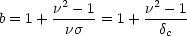(129)

(Kaiser 1984; Cole & Kaiser 1989; Mo & White 1996), where = _c / , and ² is the fractional mass variance at the redshift of interest. This formula is not perfectly accurate, but the deviations may be traced to the fact that the Press-Schechter formula for the number density of haloes (which is assumed in deriving the bias) is itself systematically in error; see Sheth & Tormen (1999).

If we do not wish to assume that the number of galaxies in a halo of mass M is strictly proportional to M, we are in effect giving haloes a mass-dependent weight, as was first considered by Jing, Mo & Börner (1998). A simple but instructive model for this is

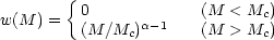(130)

A model in which mass traces light would have M_c 0 and = 1. We will show below that, empirically, we should choose < 1.

The bias formula applies to haloes of a given , i.e. of a given mass, so the effect of mass-dependent weights is

(131)

Where F( > ) is the fraction of the mass in haloes exceeding a given ; dF / d exp(- ² / 2) according to Press-Schechter theory. The total model for the galaxy power spectrum is then

(132)

where

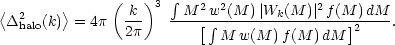(133)

The key ingredient needed to make this machinery work is the occupation number, which in principle needs to be calculated via a detailed numerical model of galaxy formation. However, for a given assumed background cosmology, the answer may be determined empirically. Galaxy redshift surveys have been analyzed via grouping algorithms similar to the `friends-of-friends' method widely employed to find virialized clumps in N-body simulations. With an appropriate correction for the survey limiting magnitude, the observed number of galaxies in a group can be converted to an estimate of the total stellar luminosity in a group. This allows a determination of the All Galaxy System (AGS) luminosity function: the distribution of virialized clumps of galaxies as a function of their total luminosity, from small systems like the Local Group to rich Abell clusters.

The AGS function for the CfA survey was investigated by Moore, Frenk & White (1993), who found that the result in blue light was well described by

(134)

where ^* = 0.00126 h³ Mpc^-3, = 1.34, = 2.89; the characteristic luminosity is L^* = 7.6 × 10¹⁰ h^-2 L. One notable feature of this function is that it is rather flat at low luminosities, in contrast to the mass function of dark-matter haloes (see Sheth & Tormen 1999). It is therefore clear that any fictitious galaxy catalogue generated by randomly sampling the mass is unlikely to be a good match to observation. The simplest cure for this deficiency is to assume that the stellar luminosity per virialized halo is a monotonic, but nonlinear, function of halo mass. The required luminosity-mass relation is then easily deduced by finding the luminosity at which the integrated AGS density ( > L) matches the integrated number density of haloes with mass > M. The result is shown in figure 14.

Figure 14. The empirical luminosity-mass relation required to reconcile the observed AGS luminosity function with two variants of CDM. L* is the characteristic luminosity in the AGS luminosity function (L* = 7.6 × 1010 h-2 L). Note the rather flat slope around M = 1013 to 1014 h-1 M, especially for CDM.

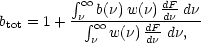
We can now calculate the halo-based galaxy power spectrum and use semi-realistic occupation numbers, N, as a function of mass. This is needs a little care at small numbers, however, since the number of haloes with occupation number unity affects the correlation properties. These haloes contribute no correlated pairs, so they simply dilute the signal from the haloes with N 2. This means that we need in principle to use different weights for the large-scale bias and the halo term:

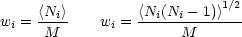(135)

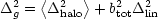
respectively (Seljak 2000). In practice, this correction has a rather small effect, provided the relation between N and M has no scatter. If, in contrast, the distribution of N for given M is assumed to obey a Poisson distribution, the small-scale clustering properties are strongly affected, and do not match the data well (Benson et al. 2000a). Finally, we need to put the galaxies in the correct location, as discussed above. If one galaxy always occupies the halo centre, with others acting as satellites, the small-scale correlations automatically follow the slope of the halo density profile, which keeps them steep. The results of this exercise are shown in figure 15. This shows that, depending on the range of halo masses chosen, the galaxies can be positively or negatively biased with respect to the mass, as expected. What is particularly interesting is that the shape of the galaxy spectrum is expected to differ from that of the mass. For an appropriate mass range, the galaxy power spectrum can be very close to a power law, which has been a long-standing puzzle to explain. Interestingly, the power-law should not be perfect; small deviations have long been suspected, and were confirmed by Hawkins et al. (2002) and Zehavi et al. (2003). The inflection is at a scale of ~ 0.5 h Mpc^-1, as expected from the halo model. Figure 15 also shows that the results of this simple model are encouragingly similar to the scale-dependent bias found in the detailed calculations of Benson et al. (2000a), shown in figure 11. There are thus grounds for optimism that we may be starting to attain a physical understanding of the origin of galaxy bias.

Figure 15. The power spectrum predicted for the halo model, for the flat m = 0.3, = 0.2, 8 = 0.8 case. The halo occupation numbers are predicted according to a simple two-parameter model, in which haloes are only included above some minimum value, Mmin, and receive a weight M. A model with `mass traces light' would have Mmin = 0 and = 1. Motivated by the results on abundances of groups, we choose = 0.5. Results are shown for Mmin in the range 109 (lowest) to 1014 h-1 M (highest). The mass power spectrum is shown as a dashed line (linear theory) and as points (nonlinear). The second panel shows the scale-dependent relative bias, i.e. the square root of the ratio between galaxy and mass power spectra. The dashed lines show the bias with respect to linear theory. The final panel shows the ratio to the canonical power-law spectrum; for Mmin in the region of 1012 h-1 M, the result is within about 10% of a perfect power law over a factor 300 in scale.