15.3. THE "WORLD PICTURE" AND SOURCE EVOLUTION

The interval during which radio observations have been made is much shorter than the active lifetimes of individual sources and the time scales on which populations of radio sources evolve, so at best the data can give only a "world picture" covering the surface of our past light cone. The luminosity functions, size distributions, etc. of different source populations at different lookback times can be compared to reveal evolution, but we cannot directly observe any changes actually taking place. One consequence of this limitation is illustrated by Figure 15.1, showing the radio luminosity functions of elliptical galaxies at two different epochs. The luminosity functions do not overlap, so cosmological evolution must occur. The arrows in Figure 15.1(a) indicate one way in which the data might be interpreted - the comoving density _m of sources was higher in the past, with the greatest changes being experienced by the most luminous sources. Such evolution is called "luminosity-dependent density evolution," a term that suggests an evolutionary mechanism capable of distinguishing between weak and strong sources. The arrows in Figure 15.1(b) show a very different interpretation of the same two luminosity functions - the luminosities of all sources were higher in the past, by an amount independent of luminosity. This "luminosity evolution" interpretation is consistent with evolutionary mechanisms that affect weak and strong sources alike. Since the active lifetimes of individual radio sources are generally shorter than the evolutionary time scales, which are, in turn, shorter than the ages of elliptical galaxies, descriptions of evolution based on associating points or features in the luminosity functions from different epochs probably oversimplify the actual changes occurring on the individual source level. In any case, the data cannot distinguish between them.

Figure 15.1. The 1.4-GHz luminosity functions of elliptical radio galaxies at z = 0 and z = 0.8 with arrows illustrating (a) luminosity-dependent density evolution and (b) pure luminosity evolution. These particular luminosity functions are from the "shell model" described in Section 15.9. Abscissas: log luminosity (W Hz-1). Ordinates: log comoving density (mag-1 Mpc-3).

Because luminosity functions _m(L | z) have dimensions of comoving source density, evolution has historically been described in terms of density changes. The "evolution function"

(15.8)

is an example. Consequently, there is a widespread misconception that the data imply "luminosity-dependent density evolution," leading to unjustified conclusions like "In view of the lack of evolution of the low-luminosity sources, it seems implausible that their spectra should change with redshift." Even though the evolution function completely specifies the changes of mean source density with luminosity and epoch, it cannot completely describe the course of evolution.

Existing data do not even determine our world picture completely. The "generalized luminosity function" _m(L, , .... | z, ) of sources with luminosity L, spectral index , and other relevant properties (e.g., type of galaxy) indicated by ... at redshift z and frequency is only partially determined. Most sources in the flux-limited sample found by any single radio survey complete to some level S are confined to a narrow diagonal band in the luminosity-redshift plane (Figure 15.2). Known radio sources span ten decades in luminosity and five in redshift, so surveys with a wide range of limiting flux densities S made with a number of different radio telescopes are needed to fill in the (L, z)-plane. More difficult than this is obtaining the optical identifications and redshifts needed to locate individual sources on the (L, z)-plane. Spectroscopic redshifts are available for most sources with S 2 Jy at = 1.4 GHz, but fainter sources with known S and unknown z could lie almost anywhere on the diagonal lines of constant S. The Leiden-Berkeley Deep Survey (Windhorst 1984, Windhorst et al. 1984b, Kron et al. 1985, Windhorst et al. 1985) is a major project to find sources as faint as S 1 mJy at = 1.4 GHz, identify nearly all of them on very deep photographic plates or CCD images and obtain photometric or spectroscopic redshifts. Efforts like this should eventually yield a direct determination of the generalized luminosity function, but until then we are limited to making models that use known radio sources with only weak constraints on their redshift distributions to extrapolate into unknown regions of the (L, z)-plane. The available data are presented in Section 15.4 and some models in Section 15.5.

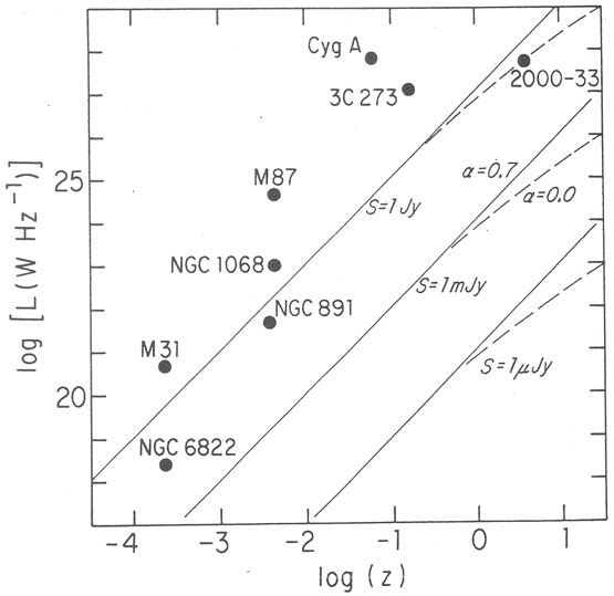Figure 15.2. Luminosities and redshifts of representative radio sources found at = 1.4 GHz. Most nearby sources with L < 1023 W Hz-1 are associated with spiral galaxies. The faintest are found in dwarf irregulars like NGC 6822; the luminosity of M31 is typical for full-sized spiral galaxies. An unusually high star formation rate probably accounts for the relatively high radio luminosity of NGC 891, and the Seyfert/starburst galaxy NGC 1068 is the strongest radio emitter of the nearby spiral galaxies. Elliptical galaxies such as M87 dominate the radio-source population at higher powers, reaching L 1028 W Hz-1). in the case of Cygnus A. Radio-selected quasars are concentrated near the upper end of this luminosity range and have known redshifts between z = 0.158 (3C273) and z = 3.78 (2000-33). Lines of constant flux density are shown for sources with spectral indices = 0.7 (solid lines) and = 0.0 (broken curves) in an Einstein-de Sitter universe ( = 1) with H0 = 100 km s-1 Mpc-1. Nearly all radio galaxies selected at = 1.4 GHz have spectral indices near = 0.7, while many quasars have 0. The faintest discrete sources detected at = 1.4 GHz have flux densities S 100 µJy and the sky density of sources as faint as S 10 µJy has been estimated statistically. Abscissa: log redshift. Ordinate: log spectral luminosity (W Hz-1).