15.6.3. Models of the Angular Size-Flux Density Relation

All evolutionary models of the observed <> - S relation (e.g., Figure 15.13) require as an input one of the models for the evolving radio luminosity function described in Section 15.5. Some estimate of the linear size distribution of sources covering a wide luminosity range (e.g., Figure 15.14) is also needed. The first detailed model (Kapahi 1975) was based on a luminosity function similar to that derived by Longair (1966). The approximation was made that the projected linear size d of a radio source is independent of its luminosity L, and a parametric "local" size distribution was obtained by a fit to the size distribution of low-redshift (z < 0.3) 3CR sources. Power law size evolution in which source sizes vary as d = d₀(1 + z)^-N was tried, and the value N 1.5 gave the best fit to the <> - S data for sources stronger than S 1 Jy at 178 MHz.

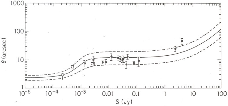Figure 15.13. Median angular size as a function of 1.4-GHz flux density. The filled circles are from the compilation by Windhorst et al. (1984); the open circles and the upper limit are from the Coleman and Condon (1985) high-resolution VLA survey. The solid line is the median angular size from the Coleman and Condon (1985) model ( = 1, no size evolution), while the dashed lines mark the 60th- and 40th-percentile angular sizes. Abscissa: flux density (Jy). Ordinate: median angular size (arcsec).

The <> - S relation was extended to S 0.1 Jy at 408 MHz by Downes et al. (1981). Their analysis was based on the improved Wall et al. (1980) radio luminosity functions. Instead of deriving a size distribution function, they assumed that individual 3CR sources are representative of the overall population of sources dominating the relevant epoch. Sources in their 3CR "parent population" were assigned weights by the weighted 1 / V'_m, method used to calculate the local luminosity function of an evolving population (Section 15.4.1). This method should automatically account for any possible correlation between linear size and luminosity in the parent sample, but spreading the parent population over a number of luminosity bins increases the statistical uncertainties in each. Also, the 3CR parent population does not correct for possible morphological differences between the 3CR sources and sources appearing elsewhere in the (L, z)-plane. If there is a substantial population of steep-spectrum compact sources (compact sources with steep spectra at high frequencies but relatively flat spectra at lower frequencies) among the faint (S < 0.1 Jy) high-redshift sources found at 408 MHz, it will be better represented in a (lower-redshift) parent population selected at some frequency higher than 408 MHz (e.g., Fielden et al. 1983, Allington-Smith 1984). Although Downes et al. (1981) found no value of the evolution exponent N reproduced the data with the 3CR parent sample, Kapahi and Subrahmanya (1982) used the same methods and data to find acceptable fits in the range 1 < N < 1.5. Kapahi et al. (1987) attribute this discrepancy to a computational oversight by Downes et al. (1981). Using a parent sample selected at = 2.7 GHz with the Peacock and Gull (1981) multi-frequency luminosity functions to predict the <> - S relation at other frequencies, Fielden et al. (1983) and Allington-Smith (1984) obtained good fits in the range 0.05 to 1 Jy at 408 MHz for 1 < N < 1.5, but the stronger sources could not be accommodated simultaneously. Finally, Kapahi et al. (1987) modeled the <> - S relation above S 0.1 Jy at 408 MHz using a variety of luminosity functions and parent populations selected at 178, 1400, and 2700 MHz. They concluded that size evolution is always required.

Most faint (S < 1 Jy at = 1.4 GHz) sources probably have redshifts in the range 0.3 < z < 3 for which the angular-size distance D is nearly constant if = 1 (Figure 15.15). Without size evolution, changes in angular size with flux density reflect changes in linear size, not redshift. Flux density correlates more strongly with luminosity than with redshift for S < 1 Jy, so the flat portion of the <> - S curve (Figure 15.13) can easily be matched without evolution if there is no correlation of linear size with luminosity (Figure 15.14). Conversely, models requiring evolution to fit this flat region generally have parent populations in which low-luminosity sources have larger median linear sizes than high-luminosity sources. The rather sharp drop in <> below S 1 mJy at = 1.4 GHz can be explained only by a correspondingly sharp drop in the median linear size of sub-mJy sources (Coleman and Condon 1985). This occurs naturally if the faintest sources are confined to the disks of spiral galaxies.

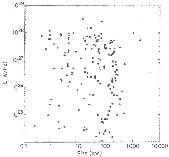Figure 15.14. Projected linear size distribution of sources stronger than S = 2 Jy at = 1.4 GHz (From Coleman and Condon 1985) calculated for = 1. The correlation of size with luminosity is weak at best. Abscissa: projected linear size (kpc). Ordinate: 1.4-GHz luminosity (W Hz-1).

All of the models above have trouble matching the rather steep rise of <> at high flux densities. This difficulty may be caused by the variation of with the dynamic range of the measurements. Using ^* instead of for all sources reduces the rise above S 1 Jy to the point that it can be fit without size evolution (Coleman 1985), although size evolution with N 1 is still quite acceptable - the <> - S relation is just not very sensitive to size evolution.