


9.1. Mapping Hydrogen Before Reionization
The small residual fraction of free electrons after cosmological
recombination coupled the temperature of the cosmic gas to that of the
cosmic microwave background (CMB) down to a redshift, z ~ 200
[284].
Subsequently, the gas temperature dropped adiabatically as
Tgas
 (1 +
z)2 below the CMB temperature
T
(1 +
z)2 below the CMB temperature
T (1 + z). The gas heated up again after being exposed to the
photo-ionizing
ultraviolet light emitted by the first stars during the reionization
epoch at z < 20. Prior to the formation of the first
stars, the cosmic neutral hydrogen must have resonantly absorbed the CMB
flux through its spin-flip 21cm transition
[131,
323,
367,
404].
The linear density fluctuations at that time should have imprinted
anisotropies on the CMB sky at an observed wavelength of
(1 + z). The gas heated up again after being exposed to the
photo-ionizing
ultraviolet light emitted by the first stars during the reionization
epoch at z < 20. Prior to the formation of the first
stars, the cosmic neutral hydrogen must have resonantly absorbed the CMB
flux through its spin-flip 21cm transition
[131,
323,
367,
404].
The linear density fluctuations at that time should have imprinted
anisotropies on the CMB sky at an observed wavelength of
 = 21.12[(1 +
z) / 100] meters. We
discuss these early 21cm fluctuations mainly for pedagogical purposes.
Detection of the earliest 21cm signal will be particularly challenging
because the foreground sky brightness rises as
2.5 at long
wavelengths in addition to the standard
1/2 scaling
of the
detector noise temperature for a given integration time and fractional
bandwidth. The discussion in this section follows Loeb & Zaldarriaga
(2004)
[226].
= 21.12[(1 +
z) / 100] meters. We
discuss these early 21cm fluctuations mainly for pedagogical purposes.
Detection of the earliest 21cm signal will be particularly challenging
because the foreground sky brightness rises as
2.5 at long
wavelengths in addition to the standard
1/2 scaling
of the
detector noise temperature for a given integration time and fractional
bandwidth. The discussion in this section follows Loeb & Zaldarriaga
(2004)
[226].
 |
Figure 53. The 21cm transition of hydrogen. The higher energy level the spin of the electron (e-) is aligned with that of the proton (p+). A spin flip results in the emission of a photon with a wavelength of 21cm (or a frequency of 1420MHz). |
We start by calculating the history of the spin temperature, Ts, defined through the ratio between the number densities of hydrogen atoms in the excited and ground state levels, n1 / n0 = (g1/ g0)exp{-T* / Ts},
 |
(154) |
where subscripts 1 and 0 correspond to the excited and
ground state levels of the 21cm transition, (g1 /
g0) = 3 is the ratio of
the spin degeneracy factors of the levels, nH =
(n0 + n1)
(1 + z)3 is the total hydrogen density, and
T* = 0.068K is the
temperature corresponding to the energy difference between the levels. The
time evolution of the density of atoms in the ground state is given by,
 |
(155) |
where a(t) = (1 + z)-1 is the cosmic
scale factor, A's and B's are the Einstein rate
coefficients, C's are the collisional rate coefficients, and
I is the blackbody intensity in the Rayleigh-Jeans tail of the CMB, namely
I
= 2kT /
2 with
= 21 cm
[306].
Here a dot denotes a time-derivative. The
0
is the blackbody intensity in the Rayleigh-Jeans tail of the CMB, namely
I
= 2kT /
2 with
= 21 cm
[306].
Here a dot denotes a time-derivative. The
0  1 transition rates
can be related to the 1
0 transition rates by the requirement that in
thermal equilibrium with Ts =
T = Tgas, the right-hand-side of
Eq. (155) should vanish with the collisional terms balancing
each other separately from the radiative terms. The Einstein coefficients
are A10 = 2.85 × 10⁻¹⁵ s-1,
B10 =
(3 /
2hc) A10 and B01 =
(g1 / g0)B10
[131,
306].
The collisional de-excitation rates can be written as
C10 = 4/3
1 transition rates
can be related to the 1
0 transition rates by the requirement that in
thermal equilibrium with Ts =
T = Tgas, the right-hand-side of
Eq. (155) should vanish with the collisional terms balancing
each other separately from the radiative terms. The Einstein coefficients
are A10 = 2.85 × 10⁻¹⁵ s-1,
B10 =
(3 /
2hc) A10 and B01 =
(g1 / g0)B10
[131,
306].
The collisional de-excitation rates can be written as
C10 = 4/3
 (1 - 0)
nH, where
(1 - 0) is tabulated as
a function of Tgas
[11,
406].
(1 - 0)
nH, where
(1 - 0) is tabulated as
a function of Tgas
[11,
406].
Equation (155) can be simplified to the form,
 |
(156) |
where 
 n0 /
nH, H
n0 /
nH, H
 H0
(
H0
( m)1/2(1 + z)3/2 is
the Hubble parameter at high redshifts
(with a present-day value of H0), and
m is the
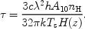
density parameter of matter. The upper panel of
Fig. 54 shows the results
of integrating Eq. (156). Both the spin temperature and the
kinetic temperature of the gas track the CMB temperature down to
z ~ 200. Collisions are efficient at coupling
Ts and Tgas down to
z ~ 70 and so the spin temperature follows the kinetic temperature
around that redshift. At much lower redshifts, the Hubble expansion makes
the collision rate subdominant relative the radiative coupling rate to the
CMB, and so Ts tracks T
again. Consequently, there is a
redshift window between 30 < z < 200, during which the
cosmic hydrogen absorbs the CMB flux at its resonant 21cm
transition. Coincidentally, this redshift interval precedes the appearance
of collapsed objects
[23]
and so its signatures are not contaminated by
nonlinear density structures or by radiative or hydrodynamic feedback
effects from stars and quasars, as is the case at lower redshifts
[404].
m)1/2(1 + z)3/2 is
the Hubble parameter at high redshifts
(with a present-day value of H0), and
m is the
density parameter of matter. The upper panel of
Fig. 54 shows the results
of integrating Eq. (156). Both the spin temperature and the
kinetic temperature of the gas track the CMB temperature down to
z ~ 200. Collisions are efficient at coupling
Ts and Tgas down to
z ~ 70 and so the spin temperature follows the kinetic temperature
around that redshift. At much lower redshifts, the Hubble expansion makes
the collision rate subdominant relative the radiative coupling rate to the
CMB, and so Ts tracks T
again. Consequently, there is a
redshift window between 30 < z < 200, during which the
cosmic hydrogen absorbs the CMB flux at its resonant 21cm
transition. Coincidentally, this redshift interval precedes the appearance
of collapsed objects
[23]
and so its signatures are not contaminated by
nonlinear density structures or by radiative or hydrodynamic feedback
effects from stars and quasars, as is the case at lower redshifts
[404].
 |
Figure 54. Upper panel: Evolution of
the gas, CMB and spin temperatures
with redshift [4]. Lower panel: dTb /
d |
During the period when the spin temperature is smaller than the CMB temperature, neutral hydrogen atoms absorb CMB photons. The resonant 21cm absorption reduces the brightness temperature of the CMB by,
 |
(157) |
where the optical depth for resonant 21cm absorption is,
 |
(158) |
Small inhomogeneities in the hydrogen density
 H
(nH -
H
(nH -
 H) /
H result in
fluctuations of the 21cm absorption
through two separate effects. An excess of neutral hydrogen directly
increases the optical depth and also alters the evolution of the spin
temperature. For now, we ignore the additional effects of peculiar
velocities (Bharadwaj & Ali 2004
[41];
Barkana & Loeb 2004
[27])
as well as fluctuations in the gas kinetic temperature due to the
adiabatic compression (rarefaction) in overdense (underdense) regions
[29].
Under these approximations, we can write an equation for the resulting
evolution of
fluctuations,
H) /
H result in
fluctuations of the 21cm absorption
through two separate effects. An excess of neutral hydrogen directly
increases the optical depth and also alters the evolution of the spin
temperature. For now, we ignore the additional effects of peculiar
velocities (Bharadwaj & Ali 2004
[41];
Barkana & Loeb 2004
[27])
as well as fluctuations in the gas kinetic temperature due to the
adiabatic compression (rarefaction) in overdense (underdense) regions
[29].
Under these approximations, we can write an equation for the resulting
evolution of
fluctuations,
 |
(159) |
leading to spin temperature fluctuations,
 |
(160) |
The resulting brightness temperature fluctuations can be related to the derivative,
 |
(161) |
The spin temperature fluctuations
Ts /
Ts are proportional to
the density fluctuations and so we define,
 |
(162) |
through
Tb = (d Tb /
d H)
H. We ignore
fluctuations in Cij due to
fluctuations in Tgas which are very small
[11].
Figure 54 shows dTb /
dH as
a function of redshift, including
the two contributions to dTb /
dH,
one originating directly from density fluctuations and the second from
the associated changes in the spin temperature
[323].
Both contributions have the same sign, because
an increase in density raises the collision rate and lowers the spin
temperature and so it allows Ts to better track Tgas. Since
H grows with
time as H
a, the signal
peaks at z ~ 50, a
slightly lower redshift than the peak of dTb /
dH.
Next we calculate the angular power spectrum of the brightness temperature
on the sky, resulting from density perturbations with a power spectrum
P(k),
 |
(163) |
where
H(k)
is the Fourier
tansform of the hydrogen density field, k is the comoving wavevector,
and < … > denotes an ensemble average (following the
formalism described in
[404]).
The 21cm brightness temperature observed at a frequency
corresponding to a distance
r along the line of sight, is given by
 |
(164) |
where n denotes the direction of
observation, W(r) is a narrow function of r that
peaks at the distance corresponding to
. The details of this function
depend on the characteristics of the experiment. The brightness
fluctuations in Eq. 164
can be expanded in spherical harmonics with expansion coefficients
alm().
The angular power spectrum of map
Cl()
= <
|alm()|2 > can be expressed in
terms of the 3D power spectrum of fluctuations in the density
P(k),
 |
(165) |
Our calculation ignores inhomogeneities in the hydrogen ionization
fraction, since they freeze at the earlier recombination epoch (z ~
103) and so their amplitude is more than an order of
magnitude smaller than
H at z
< 100. The gravitational
potential perturbations induce a redshift distortion effect that is of
order ~ (H / ck)2 smaller than
H for the
high - l modes of interest here.
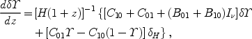
Figure 55 shows the angular power spectrum at
various redshifts.
The signal peaks around z ~ 50 but maintains a substantial
amplitude over the full range of 30 < z < 100.
The ability to probe the small scale power of density fluctuations is only
limited by the Jeans scale, below which the dark matter inhomogeneities are
washed out by the finite pressure of the gas. Interestingly, the
cosmological Jeans mass reaches its minimum value, ~ 3 ×
104
M ,
within the redshift interval of interest here which
corresponds to modes of angular scale ~ arcsecond on the sky. During
the epoch of reionization, photoionization heating raises the Jeans mass by
several orders of magnitude and broadens spectral features, thus limiting
the ability of other probes of the intergalactic medium, such as the
Ly
,
within the redshift interval of interest here which
corresponds to modes of angular scale ~ arcsecond on the sky. During
the epoch of reionization, photoionization heating raises the Jeans mass by
several orders of magnitude and broadens spectral features, thus limiting
the ability of other probes of the intergalactic medium, such as the
Ly forest, from
accessing the same very low mass scales. The 21cm
tomography has the additional advantage of probing the majority of the
cosmic gas, instead of the trace amount (~ 10-5) of neutral
hydrogen probed by the Ly
forest after reionization. Similarly to
the primary CMB anisotropies, the 21cm signal is simply shaped by gravity,
adiabatic cosmic expansion, and well-known atomic physics, and is not
contaminated by complex astrophysical processes that affect the
intergalactic medium at z < 30.
forest, from
accessing the same very low mass scales. The 21cm
tomography has the additional advantage of probing the majority of the
cosmic gas, instead of the trace amount (~ 10-5) of neutral
hydrogen probed by the Ly
forest after reionization. Similarly to
the primary CMB anisotropies, the 21cm signal is simply shaped by gravity,
adiabatic cosmic expansion, and well-known atomic physics, and is not
contaminated by complex astrophysical processes that affect the
intergalactic medium at z < 30.
 |
Figure 55. Angular power spectrum of 21cm anisotropies on the sky at various redshifts. From top to bottom, z = 55,40,80,30,120,25,170. |
Characterizing the initial fluctuations is one of the
primary goals of observational cosmology, as it offers a window into the
physics of the very early Universe, namely the epoch of inflation during
which the fluctuations are believed to have been produced.
In most models of inflation, the evolution of the Hubble parameter during
inflation leads to departures from a scale-invariant spectrum that are of
order 1/Nefold with Nefold ~ 60
being the number of e - folds between the time when the scale of
our horizon was of order the horizon during inflation and the end of
inflation
[218].
Hints that the standard
 CDM model may have
too much power on galactic scales have inspired
several proposals for suppressing the power on small scales. Examples
include the possibility that the dark matter is warm and it decoupled while
being relativistic so that its free streaming erased small-scale power
[48],
or direct modifications of inflation that produce a cut-off in
the power on small scales
[192].
An unavoidable collisionless component of the cosmic mass budget beyond
CDM, is provided by massive neutrinos (see
[198]
for a review). Particle physics experiments
established the mass splittings among different species which translate
into a lower limit on the fraction of the dark matter accounted for by
neutrinos of f
> 0.3 %, while current constraints based on galaxies
as tracers of the small scale power imply
f
< 12 %
[360].
CDM model may have
too much power on galactic scales have inspired
several proposals for suppressing the power on small scales. Examples
include the possibility that the dark matter is warm and it decoupled while
being relativistic so that its free streaming erased small-scale power
[48],
or direct modifications of inflation that produce a cut-off in
the power on small scales
[192].
An unavoidable collisionless component of the cosmic mass budget beyond
CDM, is provided by massive neutrinos (see
[198]
for a review). Particle physics experiments
established the mass splittings among different species which translate
into a lower limit on the fraction of the dark matter accounted for by
neutrinos of f
> 0.3 %, while current constraints based on galaxies
as tracers of the small scale power imply
f
< 12 %
[360].
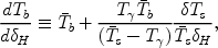
Figure 56 shows the 21cm power spectrum for various
models that differ in their level of small scale power. It is clear that a
precise measurement of the 21cm power spectrum will dramatically improve
current constraints on alternatives to the standard
CDM spectrum.
 |
Figure 56. Upper panel: Power
spectrum of 21cm anisotropies at z = 55
for a |
The 21cm signal contains a wealth of information about the
initial fluctuations. A full sky map at a single photon
frequency measured up to lmax, can
probe the power spectrum up to kmax ~
(lmax / 104) Mpc-1. Such a map
contains lmax2 independent samples. By
shifting the photon frequency, one may obtain many independent measurements
of the power. When measuring a mode l, which corresponds to a
wavenumber k ~ l / r, two maps at different photon
frequencies will be independent if they are separated in radial distance
by 1 / k. Thus, an experiment that covers a spatial range
 r can probe
a total of
k r ~
l
r / r
independent maps. An experiment that detects the 21cm signal
over a range
centered on a frequency
, is
sensitive to
r / r
~ 0.5 (
/
)(1 +
z)-1/2, and so it
measures a total of N21cm ~ 3 ×
1016 (lmax / 106)3
(
/
)
(z / 100)-1/2 independent samples.
r can probe
a total of
k r ~
l
r / r
independent maps. An experiment that detects the 21cm signal
over a range
centered on a frequency
, is
sensitive to
r / r
~ 0.5 (
/
)(1 +
z)-1/2, and so it
measures a total of N21cm ~ 3 ×
1016 (lmax / 106)3
(
/
)
(z / 100)-1/2 independent samples.
This detection capability cannot be reproduced even remotely by other
techniques. For example, the primary CMB anisotropies are damped on small
scales (through the so-called Silk damping), and probe only modes with
l
 3000 (k
0.2 Mpc-1). The
total number of modes
available in the full sky is Ncmb = 2
lmax2 ~ 2 ×
107 (lmax / 3000)2, including both
temperature and polarization information.
3000 (k
0.2 Mpc-1). The
total number of modes
available in the full sky is Ncmb = 2
lmax2 ~ 2 ×
107 (lmax / 3000)2, including both
temperature and polarization information.
The sensitivity of an experiment depends strongly on its particular design,
involving the number and distribution of the antennae for an
interferometer. Crudely speaking, the uncertainty in the measurement of
[l(l + 1)Cl /
2 ]1/2 is dominated
by noise,
N,
which is controlled by the sky brightness
I
at the observed frequency
[404],
]1/2 is dominated
by noise,
N,
which is controlled by the sky brightness
I
at the observed frequency
[404],
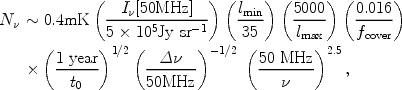 |
(166) |
where lmin is the minimum observable l as
determined by the field of view of the instruments,
lmax is the maximum observable
l as determined by the maximum separation of the antennae,
fcover is the fraction of the array area thats
is covered by telescopes,
t0 is the observation time and
is the frequency range over
which the signal can be detected. Note that the assumed sky temperature of
0.7 × 10⁴ K at
= 50 MHz (corresponding to
z ~ 30) is more than
six orders of magnitude larger than the signal. We have already included
the fact that several independent maps can be produced by varying the
observed frequency. The numbers adopted above are appropriate for the
inner core of the LOFAR array
(http://www.lofar.org),
planned for initial operation in 2006. The predicted signal is ~ 1 mK,
and so a year of integration or an increase in the covering fraction are
required to observe it with LOFAR. Other experiments whose goal is
to detect 21cm fluctuations from the subsequent epoch of reionization at
z ~ 6-12 (when ionized bubbles exist and the fluctuations are larger)
include the Mileura Wide-Field Array (MWA;
http://web.haystack.mit.edu/arrays/MWA/),
the Primeval Structure Telescope
(PAST;
http://arxiv.org/abs/astro-ph/0502029),
and in the more
distant future the Square Kilometer Array (SKA;
http://www.skatelescope.org).
The main challenge in detecting the
predicted signal from higher redshifts involves its appearance at low
frequencies where the sky noise is high. Proposed space-based instruments
[194]
avoid the terrestrial radio noise and the increasing
atmospheric opacity at <
20 MHz (corresponding to z > 70).
 |
Figure 57. Prototype of the tile design for the Mileura Wide-Field Array (MWA) in western Australia, aimed at detecting redshifted 21cm from the epoch of reionization. Each 4m×4m tile contains 16 dipole antennas operating in the frequency range of 80 - 300MHz. Altogether the initial phase of MWA (the so-called "Low-Frequency Demostrator") will include 500 antenna tiles with a total collecting area of 8000 m2 at 150MHz, scattered across a 1.5 km region and providing an angular resolution of a few arcminutes. |
The 21cm absorption is replaced by 21cm emission from neutral hydrogen as
soon as the intergalactic medium is heated above the CMB temperature by
X-ray sources during the epoch of reionization
[88].
This occurs long before reionization since the required heating requires
only a modest amount of energy, ~ 10-2 eV[(1 + z) /
30], which is three orders
of magnitude smaller than the amount necessary to ionize the Universe. As
demonstrated by Chen & Miralda-Escude (2004)
[88],
heating due the recoil of atoms as they absorb
Ly photons
[237]
is not effective; the Ly
color temperature reaches equilibrium with the
gas kinetic temperature and suppresses subsequent heating before the level
of heating becomes substantial. Once most of the cosmic hydrogen is
reionized at zreion, the 21cm signal is
diminished. The optical depth for free-free absorption after
reionization, ~ 0.1 [(1 + zreion) /
20]5/2, modifies only slightly the expected 21cm
anisotropies. Gravitational lensing should modify the power spectrum
[287] at high
l, but can be separated as in standard CMB studies (see
[326]
and references therein). The 21cm signal should be simpler to clean as it
includes the same lensing foreground in independent maps obtained at
different frequencies.
 |
Figure 58. Schematic sketch of the
evolution of the kinetic temperature
(Tk) and spin temperature (Ts) of
cosmic hydrogen. Following cosmological recombination at z ~
103, the gas temperature (orange
curve) tracks the CMB temperature (blue line;
T |
The large number of independent modes probed by the 21cm signal would provide a measure of non-Gaussian deviations to a level of ~ N21 cm-1/2, constituting a test of the inflationary origin of the primordial inhomogeneities which are expected to possess deviations > 10-6 [245].
9.2. The Characteristic Observed Size of Ionized Bubbles at the End of Reionization
 |
Figure 59. 21cm imaging of ionized bubbles during the epoch of reionization is analogous to slicing swiss cheese. The technique of slicing at intervals separated by the typical dimension of a bubble is optimal for revealing different pattens in each slice. |
The first galaxies to appear in the Universe at redshifts z > 20 created ionized bubbles in the intergalactic medium (IGM) of neutral hydrogen (H I) left over from the Big-Bang. It is thought that the ionized bubbles grew with time, surrounded clusters of dwarf galaxies [67, 143] and eventually overlapped quickly throughout the Universe over a narrow redshift interval near z ~ 6. This event signaled the end of the reionization epoch when the Universe was a billion years old. Measuring the unknown size distribution of the bubbles at their final overlap phase is a focus of forthcoming observational programs aimed at highly redshifted 21cm emission from atomic hydrogen. In this sub-section we follow Wyithe & Loeb (2004) [399] and show that the combined constraints of cosmic variance and causality imply an observed bubble size at the end of the overlap epoch of ~ 10 physical Mpc, and a scatter in the observed redshift of overlap along different lines-of-sight of ~ 0.15. This scatter is consistent with observational constraints from recent spectroscopic data on the farthest known quasars. This result implies that future radio experiments should be tuned to a characteristic angular scale of ~ 0.5° and have a minimum frequency band-width of ~ 8 MHz for an optimal detection of 21cm flux fluctuations near the end of reionization.
During the reionization epoch, the characteristic bubble size (defined here as the spherically averaged mean radius of the H II regions that contain most of the ionized volume [143]) increased with time as smaller bubbles combined until their overlap completed and the diffuse IGM was reionized. However the largest size of isolated bubbles (fully surrounded by H I boundaries) that can be observed is finite, because of the combined phenomena of cosmic variance and causality. Figure 61 presents a schematic illustration of the geometry. There is a surface on the sky corresponding to the time along different lines-of-sight when the diffuse (uncollapsed) IGM was most recently neutral. We refer to it as the Surface of Bubble Overlap (SBO). There are two competing sources for fluctuations in the SBO, each of which is dependent on the characteristic size, RSBO, of the ionized regions just before the final overlap. First, the finite speed of light implies that 21cm photons observed from different points along the curved boundary of an H II region must have been emitted at different times during the history of the Universe. Second, bubbles on a comoving scale R achieve reionization over a spread of redshifts due to cosmic variance in the initial conditions of the density field smoothed on that scale. The characteristic scale of H II bubbles grows with time, leading to a decline in the spread of their formation redshifts [67] as the cosmic variance is averaged over an increasing spatial volume. However the 21cm light-travel time across a bubble rises concurrently. Suppose a signal 21cm photon which encodes the presence of neutral gas, is emitted from the far edge of the ionizing bubble. If the adjacent region along the line-of-sight has not become ionized by the time this photon reaches the near side of the bubble, then the photon will encounter diffuse neutral gas. Other photons emitted at this lower redshift will therefore also encode the presence of diffuse neutral gas, implying that the first photon was emitted prior to overlap, and not from the SBO. Hence the largest observable scale of H II regions when their overlap completes, corresponds to the first epoch at which the light crossing time becomes larger than the spread in formation times of ionized regions. Only then will the signal photon leaving the far side of the HII region have the lowest redshift of any signal photon along that line-of-sight.
 |
Figure 60. Spectra of 19 quasars with
redshifts 5.74 < z < 6.42 from the Sloan Digital Sky
Survey
[128].
For some of the highest-redshift
quasars, the spectrum shows no transmitted flux shortward of the
Ly |
The observed spectra of some quasars beyond z ~ 6.1 show a
Gunn-Peterson trough
[163,
127]
(Fan et al. 2005
[128]),
a blank spectral region at wavelengths shorter than
Ly at the quasar
redshift, implying the presence
of H I in the diffuse IGM. The detection of Gunn-Peterson troughs
indicates a rapid change
[126,
288,
381]
in the neutral content of the IGM
at z ~ 6, and hence a rapid change in the intensity of the background
ionizing flux. This rapid change implies that overlap, and hence the
reionization epoch, concluded near z ~ 6. The most promising
observational probe
[404,
259]
of the reionization epoch is redshifted
21cm emission from intergalactic H I. Future observations using low
frequency radio arrays (e.g. LOFAR, MWA, and PAST) will allow a direct
determination of the topology and duration of the phase of bubble
overlap. In this section we determine the expected angular scale and
redshift width of the 21cm fluctuations at the SBO theoretically, and show
that this determination is consistent with current observational
constraints.
 |
Figure 61. The distances to the observed
Surface of Bubble Overlap (SBO) and Surface of
Ly |
We start by quantifying the constraints of causality and cosmic variance. First suppose we have an H II region with a physical radius R / (1 + < z >). For a 21cm photon, the light crossing time of this radius is
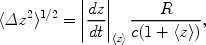 |
(167) |
where at the high-redshifts of interest
(dz / dt) = -(H0
m1/2)(1 +
z)5/2. Here, c is the speed of
light, H0 is the present-day Hubble constant,
m is the
present
day matter density parameter, and < z > is the mean redshift
of the SBO. Note that when discussing this crossing time, we are referring
to photons used to probe the ionized bubble (e.g. at 21cm), rather than
photons involved in the dynamics of the bubble evolution.
Second, overlap would have occurred at different times in different regions
of the IGM due to the cosmic scatter in the process of structure formation
within finite spatial volumes
[67].
Reionization should be completed
within a region of comoving radius R when the fraction of mass
incorporated into collapsed objects in this region attains a certain
critical value, corresponding to a threshold number of ionizing photons
emitted per baryon. The ionization state of a region is governed by the
enclosed ionizing luminosity, by its over-density, and by dense pockets of
neutral gas that are self shielding to ionizing radiation. There is an
offset
[67]
z between the
redshift when a region of mean over-density
 R
achieves this critical collapsed fraction, and the redshift
R
achieves this critical collapsed fraction, and the redshift
 when the Universe
achieves the same collapsed fraction on average. This offset may be computed
[67]
from the expression for the collapsed fraction
[52]
Fcol within a region of over-density
R on a
comoving scale R,
when the Universe
achieves the same collapsed fraction on average. This offset may be computed
[67]
from the expression for the collapsed fraction
[52]
Fcol within a region of over-density
R on a
comoving scale R,
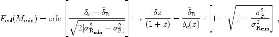 |
(168) |
where
c()
(1 + ) is the
collapse threshold for an over-density at a redshift
;
 R and
Rmin
are the variances in the power-spectrum linearly
extrapolated to z = 0 on comoving scales corresponding to the
region of interest and to the minimum galaxy mass Mmin,
respectively. The offset in the ionization redshift of a region depends
on its linear over-density,
R. As a
result, the distribution of
offsets, and therefore the scatter in the SBO may be obtained directly from
the power spectrum of primordial inhomogeneities. As can be seen from
equation (168), larger regions have a smaller scatter due to
their smaller cosmic variance.
R and
Rmin
are the variances in the power-spectrum linearly
extrapolated to z = 0 on comoving scales corresponding to the
region of interest and to the minimum galaxy mass Mmin,
respectively. The offset in the ionization redshift of a region depends
on its linear over-density,
R. As a
result, the distribution of
offsets, and therefore the scatter in the SBO may be obtained directly from
the power spectrum of primordial inhomogeneities. As can be seen from
equation (168), larger regions have a smaller scatter due to
their smaller cosmic variance.
Note that equation (168) is independent of the critical value of the collapsed fraction required for reionization. Moreover, our numerical constraints are very weakly dependent on the minimum galaxy mass, which we choose to have a virial temperature of 104 K corresponding to the cooling threshold of primordial atomic gas. The growth of an H II bubble around a cluster of sources requires that the mean-free-path of ionizing photons be of order the bubble radius or larger. Since ionizing photons can be absorbed by dense pockets of neutral gas inside the H II region, the necessary increase in the mean-free-path with time implies that the critical collapsed fraction required to ionize a region of size R increases as well. This larger collapsed fraction affects the redshift at which the region becomes ionized, but not the scatter in redshifts from place to place which is the focus of this sub-section. Our results are therefore independent of assumptions about unknown quantities such as the star formation efficiency and the escape fraction of ionizing photons from galaxies, as well as unknown processes of feedback in galaxies and clumping of the IGM.
Figure 62 displays the above two fundamental
constraints. The causality constraint (Eq. 167) is shown as the blue line,
giving a longer crossing time for a larger bubble size. This contrasts with
the constraint of cosmic variance (Eq. 168), indicated by the red
line, which shows how the scatter in formation times decreases with
increasing bubble size. The scatter in the SBO redshift and the
corresponding fluctuation scale of the SBO are given by the intersection of
these curves. We find that the thickness of the SBO is
<
z2 >1/2 ~ 0.13, and that the bubbles
which form the SBO have a
characteristic comoving size of ~ 60 Mpc (equivalent to 8.6 physical
Mpc). At z ~ 6 this size corresponds to angular scales of
 SBO ~ 0.4
degrees on the sky.
SBO ~ 0.4
degrees on the sky.
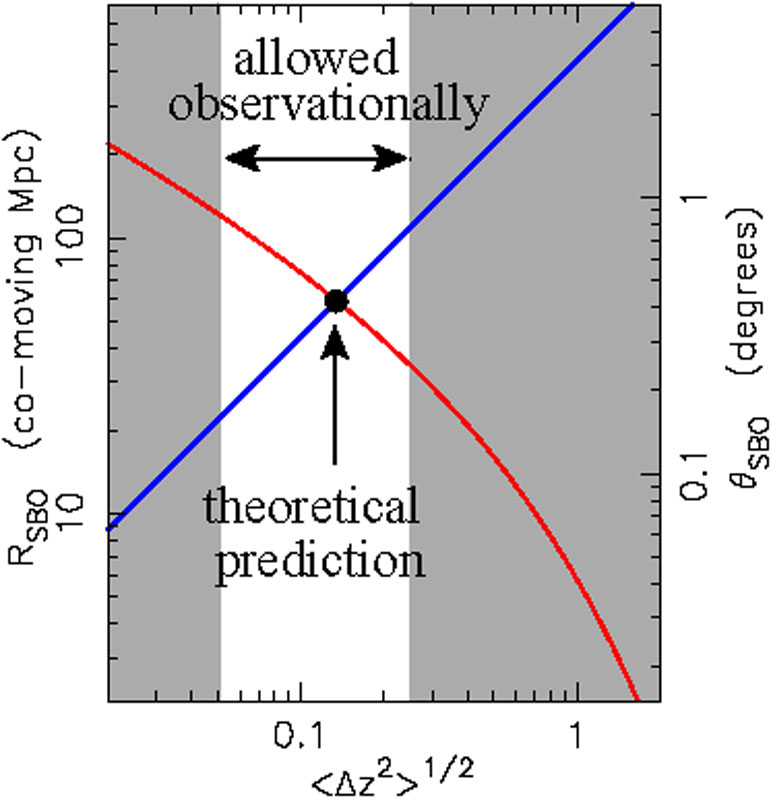 |
Figure 62. Constraints on the scatter in
the SBO redshift and
the characteristic size of isolated bubbles at the final overlap stage,
RSBO (see Fig. 1). The characteristic size of H II
regions grows
with time. The SBO is observed for the bubble scale at which the light
crossing time (blue line) first becomes smaller than the cosmic scatter in
bubble formation times (red line). At z ~ 6, the implied scale
RSBO ~ 60 comoving Mpc (or ~ 8.6 physical Mpc),
corresponds to a characteristic angular radius of
|
A scatter of ~ 0.15 in the SBO is somewhat larger than the value extracted from existing numerical simulations [152, 402]. The difference is most likely due to the limited size of the simulated volumes; while the simulations appropriately describe the reionization process within limited regions of the Universe, they are not sufficiently large to describe the global properties of the overlap phase [67]. The scales over which cosmological radiative transfer has been simulated are smaller than the characteristic extent of the SBO, which we find to be RSBO ~ 70 comoving Mpc.
We can constrain the scatter in the SBO redshift observationally using the
spectra of the highest redshift quasars. Since only a trace amount of
neutral hydrogen is needed to absorb
Ly photons, the time
where the IGM becomes Ly
transparent need not coincide with bubble
overlap. Following overlap the IGM was exposed to ionizing sources in all
directions and the ionizing intensity rose rapidly. After some time the
ionizing background flux was sufficiently high that the H I fraction fell
to a level at which the IGM allowed transmission of resonant
Ly photons. This is
shown schematically in Figure 61. The lower
wavelength limit of the Gunn-Peterson trough corresponds to the
Ly wavelength at the
redshift when the IGM started to allow transmission of
Ly photons along
that particular line-of-sight. In addition to the
SBO we therefore also define the Surface of
Ly Transmission (hereafter
SLT) as the redshift along different lines-of-sight when the diffuse IGM
became transparent to
Ly photons.
The scatter in the SLT redshift is an observable which we would like to compare with the scatter in the SBO redshift. The variance of the density field on large scales results in the biased clustering of sources [67]. H II regions grow in size around these clusters of sources. In order for the ionizing photons produced by a cluster to advance the walls of the ionized bubble around it, the mean-free-path of these photons must be of order the bubble size or larger. After bubble overlap, the ionizing intensity at any point grows until the ionizing photons have time to travel across the scale of the new mean-free-path, which represents the horizon out to which ionizing sources are visible. Since the mean-free-path is larger than RSBO, the ionizing intensity at the SLT averages the cosmic scatter over a larger volume than at the SBO. This constraint implies that the cosmic variance in the SLT redshift must be smaller than the scatter in the SBO redshift. However, it is possible that opacity from small-scale structure contributes additional scatter to the SLT redshift.
If cosmic variance dominates the observed scatter in the SLT redshift, then
based on the spectra of the three z > 6.1 quasars
[127,
381]
we would expect the scatter in the SBO redshift to satisfy
<
z2 >obs1/2 > 0.05. In
addition, analysis of the proximity effect for the size of the H
II regions around the two highest redshift quasars
[396,
251]
implies a neutral fraction that is
of order unity (i.e. pre-overlap) at z ~ 6.2-6.3, while the
transmission of Ly
photons at z < 6 implies that overlap must have completed
by that time. This restricts the scatter in the SBO to be
<
z2 >obs1/2 < 0.25. The
constraints on values for the scatter in the SBO redshift are shaded
gray in Figure 62. It is
reassuring that the theoretical prediction for the SBO scatter of
<
z2 >obs1/2 ~ 0.15, with a
characteristic scale of ~ 70 comoving Mpc, is bounded by these constraints.
The possible presence of a significantly neutral IGM just beyond the
redshift of overlap
[396,
251]
is encouraging for upcoming
21cm studies of the reionization epoch as it results in emission near an
observed frequency of 200 MHz where the signal is most readily
detectable. Future observations of redshifted 21cm line emission at 6 <
z < 6.5 with instruments such as LOFAR, MWA, and PAST, will be
able to map the three-dimensional distribution of HI at the end of
reionization. The intergalactic H II regions will imprint a 'knee' in the
power-spectrum of the 21cm anisotropies on a characteristic angular scale
corresponding to a typical isolated H II region
[404].
Our results suggest that this characteristic angular scale is large at
the end of reionization,
SBO ~ 0.5
degrees, motivating the
construction of compact low frequency arrays. An SBO thickness of
<
z2 >1/2 ~ 0.15 suggests a minimum
frequency band-width of
~ 8 MHz for experiments aiming to detect anisotropies in 21cm emission
just prior to overlap. These results will help guide the design of the next
generation of low-frequency radio observatories in the search for 21cm
emission at the end of the reionization epoch.
The full size distribution of ionized bubbles has to be calculated from a numerical cosmological simulation that includes gas dynamics and radiative transfer. The simulation box needs to be sufficiently large for it to sample an unbiased volume of the Universe with little cosmic variance, but at the same time one must resolve the scale of individual dwarf galaxies which provide (as well as consume) ionizing photons (see discussion at the last section of this review). Until a reliable simulation of this magnitude exists, one must adopt an approximate analytic approach to estimate the bubble size distribution. Below we describe an example for such a method, developed by Furlanetto, Zaldarriaga, & Hernquist (2004) [143].
The criterion for a region to be ionized is that galaxies inside of it
produce a sufficient number of ionizing photons per baryon. This condition
can be translated to the requirement that the collapsed fraction of mass in
halos above some threshold mass Mmin will exceed some
threshold, namely Fcol >
 -1.
The minimum halo mass most likely corresponds to a virial temperature of
104 K relating to the threshold
for atomic cooling (assuming that molecular hydrogen cooling is suppressed
by the UV background in the Lyman-Werner band). We would like to find the
largest region around every point that satisfies the above condition on the
collapse fraction and then calculate the abundance of ionized regions of
this size. Different regions have different values of Fcol
because their mean density is different. In the extended Press-Schechter
model (Bond et al. 1991
[52];
Lacey & Cole 1993
[212]),
the collapse fraction in a region of mean overdensity
M is
-1.
The minimum halo mass most likely corresponds to a virial temperature of
104 K relating to the threshold
for atomic cooling (assuming that molecular hydrogen cooling is suppressed
by the UV background in the Lyman-Werner band). We would like to find the
largest region around every point that satisfies the above condition on the
collapse fraction and then calculate the abundance of ionized regions of
this size. Different regions have different values of Fcol
because their mean density is different. In the extended Press-Schechter
model (Bond et al. 1991
[52];
Lacey & Cole 1993
[212]),
the collapse fraction in a region of mean overdensity
M is
 |
(169) |
where 2(M, z) is the variance of density
fluctuations on mass scale M,
min2
2(Mmin, z),
and c is the collapse threshold. This equation can be used
to derive the condition on the mean overdensity within
a region of mass M in order for it to be ionized,
 |
(170) |
where K()
= erfc-1(1 -
-1).
Furlanetto et al.
[143]
showed how to construct the mass function of ionized regions
from b in
analogy with the halo mass function (Press & Schechter 1974
[291];
Bond et al. 1991
[52]).
The barrier in equation (170) is well approximated by a linear dependence on
2,
 |
(171) |
in which case the mass function has an analytic solution (Sheth 1998 [332]),
 |
(172) |
where  is the mean mass density. This solution provides the
comoving number density of ionized bubbles with mass in the range of
(M, M + dM). The main difference of this result
from the Press-Schechter mass function is that the barrier in this case
becomes more difficult to cross on smaller scales because
B is a
decreasing function of mass
M. This gives bubbles a characteristic size. The size evolves with
redshift in a way that depends only on
and
Mmin.
is the mean mass density. This solution provides the
comoving number density of ionized bubbles with mass in the range of
(M, M + dM). The main difference of this result
from the Press-Schechter mass function is that the barrier in this case
becomes more difficult to cross on smaller scales because
B is a
decreasing function of mass
M. This gives bubbles a characteristic size. The size evolves with
redshift in a way that depends only on
and
Mmin.
One limitation of the above analytic model is that it ignores the non-local influence of sources on distant regions (such as voids) as well as the possible shadowing effect of intervening gas. Radiative transfer effects in the real Universe are inherently three-dimensional and cannot be fully captured by spherical averages as done in this model. Moreover, the value of Mmin is expected to increase in regions that were already ionized, complicating the expectation of whether they will remain ionized later. The history of reionization could be complicated and non monotonic in individual regions, as described by Furlanetto & Loeb (2005) [144]. Finally, the above analytic formalism does not take the light propagation delay into account as we have done above in estimating the characteristic bubble size at the end of reionization. Hence this formalism describes the observed bubbles only as long as the characteristic bubble size is sufficiently small, so that the light propagation delay can be neglected compared to cosmic variance. The general effect of the light propagation delay on the power-spectrum of 21cm fluctuations was quantified by Barkana & Loeb (2005) [29].
9.3. Separating the "Physics" from the "Astrophysics" of the Reionization Epoch with 21cm Fluctuations
The 21cm signal can be seen from epochs during which the cosmic gas was
largely neutral and deviated from thermal equilibrium with the cosmic
microwave background (CMB). The signal vanished at redshifts z >
200, when the residual fraction of free electrons after cosmological
recombination kept the gas kinetic temperature, Tk,
close to the CMB temperature,
T.
But during 200 > z > 30 the gas
cooled adiabatically and atomic collisions kept the spin temperature
of the hyperfine level population below
T, so that the gas appeared in absorption
[323,
226].
As the Hubble expansion
continued to rarefy the gas, radiative coupling of Ts
to T
began to dominate and the 21cm signal faded. When the first galaxies
formed, the UV photons they produced between the
Ly and Lyman
limit wavelengths propagated freely through the Universe, redshifted
into the Ly resonance,
and coupled Ts and Tk once
again through the Wouthuysen-Field
[388,
131]
effect by which the two hyperfine states are mixed through the
absorption and re-emission of a
Ly photon
[237,
96].
Emission above the Lyman limit by the same galaxies initiated the
process of reionization by creating ionized bubbles in the neutral
cosmic gas, while X-ray photons propagated farther and heated
Tk
above T throughout the Universe. Once Ts
grew larger than
T, the gas appeared in 21cm emission. The ionized
bubbles imprinted a knee in the power spectrum of 21cm fluctuations
[404],
which traced the H I topology until the process of reionization was
completed
[143].
The various effects that determine the 21cm fluctuations can be separated
into two classes. The density power spectrum probes basic cosmological
parameters and inflationary initial conditions, and can be calculated
exactly in linear theory. However, the radiation from galaxies, both
Ly radiation and
ionizing photons, involves the complex, non-linear
physics of galaxy formation and star formation. If only the sum of all
fluctuations could be measured, then it would be difficult to extract the
separate sources, and in particular, the extraction of the power spectrum
would be subject to systematic errors involving the properties of
galaxies. Barkana & Loeb (2005)
[28] showed that the unique
three-dimensional properties of 21cm measurements permit a separation of
these distinct effects. Thus, 21cm fluctuations can probe astrophysical
(radiative) sources associated with the first galaxies, while at the same
time separately probing the physical (inflationary) initial conditions of
the Universe. In order to affect this separation most easily, it is
necessary to measure the three-dimensional power spectrum of 21cm
fluctuations. The discussion in this section follows Barkana & Loeb
(2005)
[28].
Spin temperature history
As long as the spin-temperature Ts is smaller than the
CMB temperature
T = 2.725 (1 + z) K, hydrogen atoms absorb the
CMB, whereas if
Ts > T they emit
excess flux. In general, the resonant 21cm
interaction changes the brightness temperature of the CMB by
[323,
237]
Tb =
 ( Ts -
T) / (1 + z), where
the optical depth at a wavelength
= 21cm is
( Ts -
T) / (1 + z), where
the optical depth at a wavelength
= 21cm is
 |
(173) |
where nH is the number density of hydrogen, A10 = 2.85 × 10⁻¹⁵ s-1 is the spontaneous emission coefficient, xHI is the neutral hydrogen fraction, and dvr / dr is the gradient of the radial velocity along the line of sight with vr being the physical radial velocity and r the comoving distance; on average dvr / dr = H(z) / (1 + z) where H is the Hubble parameter. The velocity gradient term arises because it dictates the path length over which a 21cm photon resonates with atoms before it is shifted out of resonance by the Doppler effect [341].
For the concordance set of cosmological parameters [348], the mean brightness temperature on the sky at redshift z is
 |
(174) |
where  HI is
the mean neutral fraction of hydrogen. The spin temperature itself is
coupled to Tk
through the spin-flip transition, which can be excited by collisions
or by the absorption of
Ly photons. As a result,
the combination that appears in Tb becomes
[131]
(Ts -
T) / Ts =
[xtot / (1 + xtot)] (1 -
T / Tk ),
where xtot =
x +
xc is the sum of the radiative and
collisional threshold parameters. These parameters are
x =
4 P
T* / 27 A10
T and xc = 4
1-0(Tk) nH
T* / 3A10
T,
where P
is the Ly scattering
rate which is proportional to the
Ly intensity, and
1-0 is tabulated as a function of
Tk
[11,
406].
The coupling of the spin temperature
to the gas temperature becomes substantial when xtot
> 1.
HI is
the mean neutral fraction of hydrogen. The spin temperature itself is
coupled to Tk
through the spin-flip transition, which can be excited by collisions
or by the absorption of
Ly photons. As a result,
the combination that appears in Tb becomes
[131]
(Ts -
T) / Ts =
[xtot / (1 + xtot)] (1 -
T / Tk ),
where xtot =
x +
xc is the sum of the radiative and
collisional threshold parameters. These parameters are
x =
4 P
T* / 27 A10
T and xc = 4
1-0(Tk) nH
T* / 3A10
T,
where P
is the Ly scattering
rate which is proportional to the
Ly intensity, and
1-0 is tabulated as a function of
Tk
[11,
406].
The coupling of the spin temperature
to the gas temperature becomes substantial when xtot
> 1.
Brightness temperature fluctuations
Although the mean 21cm emission or absorption is difficult to measure due
to bright foregrounds, the unique character of the fluctuations in
Tb allows for a much easier extraction of the signal
[154,
404,
259,
260,
314].
We adopt the notation
A for the
fractional fluctuation in quantity A (with a lone
denoting
density perturbations). In general, the fluctuations in
Tb can be sourced by fluctuations in gas density
(),
Ly flux (through
x) neutral
fraction
(xHI), radial velocity gradient
(drvr), and temperature, so
we find
 |
(175) |
where the adiabatic index is
a
= 1 +
(Tk
/ ), and we define
tot
(1 + xtot) xtot. Taking the Fourier
transform, we obtain the power spectrum of each quantity; e.g., the
total power spectrum PTb
is defined by
 |
(176) |
where
Tb
(k) is the Fourier transform of
Tb,
k is the comoving wavevector,
D is the
Dirac delta function, and < ... >
denotes an ensemble average. In this analysis, we consider
scales much bigger than the characteristic bubble size and the early phase
of reionization (when
 << 1), so that the fluctuations
xHI
are also much smaller than unity. For a
more general treatment, see McQuinn et al. (2005)
[250].
<< 1), so that the fluctuations
xHI
are also much smaller than unity. For a
more general treatment, see McQuinn et al. (2005)
[250].
The separation of powers
The fluctuation
Tb
consists of a number of isotropic
sources of fluctuations plus the peculiar velocity term
-drvr. Its Fourier transform
is simply proportional to that of the density field
[191,
41],
 |
(177) |
where µ =
cos k in terms
of the angle k
of k with respect to the line of
sight. The µ2 dependence in this equation results
from taking the radial (i.e., line-of-sight) component
( µ) of
the peculiar velocity, and then the radial component
( µ) of its
gradient. Intuitively, a high-density region possesses a velocity
infall towards the density peak, implying that a photon must travel
further from the peak in order to reach a fixed relative redshift,
compared with the case of pure Hubble expansion. Thus the optical
depth is always increased by this effect in regions with
>
0. This phenomenon is most properly termed velocity
compression.
We therefore write the fluctuation in Fourier space as
 |
(178) |
where we have defined a coefficient
 by
collecting all terms
in Eq. (175), and have
also combined the terms that depend on the radiation fields of
Ly photons and
ionizing photons, respectively. We assume that these radiation fields
produce isotropic power spectra, since the physical processes that
determine them have no preferred direction in space. The total power
spectrum is
by
collecting all terms
in Eq. (175), and have
also combined the terms that depend on the radiation fields of
Ly photons and
ionizing photons, respectively. We assume that these radiation fields
produce isotropic power spectra, since the physical processes that
determine them have no preferred direction in space. The total power
spectrum is
 |
(179) |
where we have defined the power spectrum
P .
rad as the Fourier transform of the cross-correlation function,
 |
(180) |
We note that a similar anisotropy in the power spectrum has been previously derived in a different context, i.e., where the use of galaxy redshifts to estimate distances changes the apparent line-of-sight density of galaxies in redshift surveys [191, 219, 178, 133]. However, galaxies are intrinsically complex tracers of the underlying density field, and in that case there is no analog to the method that we demonstrate below for separating in 21cm fluctuations the effect of initial conditions from that of later astrophysical processes.
The velocity gradient term has also been examined for its global effect on
the sky-averaged power and on radio visibilities
[366,
41].
The other sources of 21cm perturbations are isotropic and would
produce a power spectrum PTb(k) that
could be measured by averaging
the power over spherical shells in k space. In the simple case where
= 1 and
only the density and velocity terms contribute, the
velocity term increases the total power by a factor o
< (1 + µ2)2 > = 1.87 in the
spherical average. However, instead of averaging the
signal, we can use the angular structure of the power spectrum to greatly
increase the discriminatory power of 21cm observations. We may break up
each spherical shell in k space into rings of constant
µ and
construct the observed
PTb(k,µ). Considering
Eq. (179) as a polynomial in µ, i.e.,
µ4 Pµ4 +
µ2 Pµ2 +
Pµ0, we see that the power at just
three values of µ is required in order to separate out the
coefficients of 1, µ2, and
µ4 for each k.
If the velocity compression were not present, then only the
µ-independent term (times Tb2)
would have been observed, and its separation into the five components
(Tb,
, and
three power spectra) would have been difficult and subject to
degeneracies. Once the power has been separated into three parts,
however, the µ4 coefficient
can be used to measure the density power spectrum directly, with no
interference from any other source of fluctuations. Since the overall
amplitude of the power spectrum, and its scaling with redshift, are well
determined from the combination of the CMB temperature fluctuations and
galaxy surveys, the amplitude of Pµ4
directly determines the mean brightness temperature Tb
on the sky, which measures a combination of Ts and
HI at the
observed redshift. McQuinn et al. (2005)
[250]
analysed in detail the parameters that can be
constrained by upcoming 21cm experiments in concert with future CMB
experiments such as Planck
(http://www.rssd.esa.int/index.php?project=PLANCK).
Once P(k) has been determined, the coefficients of
the µ2 term and the µ-independent
term must be used to determine the remaining unknowns,
,
P . rad(k), and
Prad(k). Since the coefficient
is
independent of k, determining it and thus breaking
the last remaining degeneracy requires only a weak additional assumption on
the behavior of the power spectra, such as their asymptotic behavior at
large or small scales. If the measurements cover Nk
values of wavenumber
k, then one wishes to determine 2 Nk + 1
quantities based on 2 Nk
measurements, which should not cause significant degeneracies when
Nk >> 1. Even without knowing
, one can
probe whether some sources of
Prad(k) are uncorrelated with
; the quantity
Pun-(k)
Pµ0 -
Pµ22 /
(4 Pµ4) equals Prad
-
P . rad2 /
P,
which receives no
contribution from any source that is a linear functional of the density
distribution (see the next subsection for an example).
Specific epochs
At z ~ 35, collisions are effective due to the high gas density,
so one can measure the density power spectrum
[226]
and the redshift evolution of nHI,
T, and Tk. At z <
35, collisions become ineffective but the first stars produce a
cosmic background of
Ly photons (i.e. photons
that redshift into
the Ly resonance) that
couples Ts to Tk. During
the period of initial
Ly coupling,
fluctuations in the Ly
flux translate into fluctuations in the 21cm brightness
[30].
This signal can be observed from z ~ 25 until the
Ly coupling is completed
(i.e., xtot >> 1) at z ~
15. At a given redshift, each atom sees
Ly photons that were
originally emitted at earlier times at rest-frame wavelengths between
Ly and the Lyman
limit. Distant sources are time retarded, and since
there are fewer galaxies in the distant, earlier Universe, each atom
sees sources only out to an apparent source horizon of ~ 100
comoving Mpc at z ~ 20. A significant portion of the flux comes
from nearby sources, because of the 1 / r2 decline of
flux with distance, and since higher Lyman series photons, which are
degraded to
Ly photons through
scattering, can only be seen from a small
redshift interval that corresponds to the wavelength interval between
two consecutive atomic levels.
There are two separate sources of fluctuations in the
Ly flux
[30].
The first is density inhomogeneities. Since gravitational
instability proceeds faster in overdense regions, the biased
distribution of rare galactic halos fluctuates much more than the
global dark matter density. When the number of sources seen by each
atom is relatively small, Poisson fluctuations provide a second source
of fluctuations. Unlike typical Poisson noise, these fluctuations are
correlated between gas elements at different places, since two nearby
elements see many of the same sources. Assuming a scale-invariant
spectrum of primordial density fluctuations, and that
x = 1
is produced at z = 20 by galaxies in dark matter halos where the gas
cools efficiently via atomic cooling,
Figure 63 shows the
predicted observable power spectra. The figure suggests that
can
be measured from the ratio Pµ2 /
Pµ4 at k > 1
Mpc-1, allowing the density-induced fluctuations in flux to be
extracted from Pµ2, while only the
Poisson fluctuations contribute to
Pun-.
Each of these components probes the
number density of galaxies through its magnitude, and the distribution
of source distances through its shape. Measurements at k > 100
Mpc-1 can independently probe Tk because of
the smoothing
effects of the gas pressure and the thermal width of the 21cm line.
 |
Figure 63. Observable power spectra during
the period of initial
Ly |
After Ly coupling and
X-ray heating are both completed, reionization continues. Since
= 1 and
Tk >> T, the
normalization of Pµ4 directly measures
the mean neutral hydrogen fraction, and one can separately probe the
density fluctuations, the neutral hydrogen fluctuations, and their
cross-correlation.
Fluctuations on large angular scales
Full-sky observations must normally be analyzed with an angular and
radial transform
[143,
314,
41],
rather than a Fourier transform which is simpler and yields more
directly the underlying 3D power spectrum
[259,
260].
The 21cm brightness fluctuations at a given redshift - corresponding to a
comoving distance r0 from the observer - can be
expanded in spherical harmonics with expansion coefficients
alm(), where
the angular power spectrum is
 |
(181) |
with
Gl(x)
Jl(x) +
( - 1)
jl(x) and Jl(x) being
a linear combination of spherical Bessel functions
[41].
In an angular transform on the sky, an angle of
radians
translates to a spherical multipole l ~ 3.5 /
. For
measurements on a screen at a comoving distance r0, a
multipole l
normally measures 3D power on a scale of k-1 ~
r0 ~
35/l Gpc for l >> 1, since r0 ~
10 Gpc at z > 10. This
estimate fails at l < 100, however, when we consider the sources
of 21cm fluctuations. The angular projection implied in
Cl involves
a weighted average (Eq. 181) that favors large scales
when l is small, but density fluctuations possess little large-scale
power, and the Cl are dominated by power around the
peak of k P(k), at a few tens of comoving Mpc.
 |
Figure 64. Effect of large-scale power on
the angular
power spectrum of 21cm anisotropies on the sky. This example shows the
power from density fluctuations and velocity compression, assuming a
warm IGM at z = 12 with Ts =
Tk >> T |
Figure 64 shows that for density and velocity
fluctuations, even
the l = 1 multipole is affected by power at k-1
> 200 Mpc only at the
2% level. Due to the small number of large angular modes available on
the sky, the expectation value of Cl cannot be
measured precisely at
small l. Figure 64 shows that this
precludes new information from being obtained on scales
k-1 > 130 Mpc using angular structure
at any given redshift. Fluctuations on such scales may be measurable using
a range of redshifts, but the required
z >
1 at z ~ 10
implies significant difficulties with foreground subtraction and with the
need to account for time evolution.