


The temperature profiles shown in the right hand panel of Fig. 10 reveal two types of clusters: those with temperature profiles falling towards the center are called cool core (CC) clusters; and clusters with no central drop of temperature are called non-cool core, NCC clusters. While the former also have high densities in their cores which implies short cooling times for the central ICM, typically one or two orders of magnitude smaller than the Hubble time, the NCC clusters have usually central cooling times exceeding the Hubble time. This observation implies that the ICM plasma should cool and condense in the CC clusters in the absence of any heat source, which could balance the cooling. Theoretical considerations focussed on the consequences of cooling without heating lead to the so-called "cooling flow" scenario (Fabian & Nulsen 1977, Fabian 1994), which predicts mass deposition in the centers of some clusters at a rate of up to hundreds to thousands of solar masses a year. In general more than half of the clusters in the nearby Universe should have cooling flows in this model (Peres et al. 1998), where the exact fractional number depends to some degree on the definition of a cooling flow.
Interestingly, in particular in the context of this review, the cooling
flow model leads to the prediction of very specific and testable
spectral signatures of a steady state cooling flow. Looking at the
plasma distribution in this scenario in temperature space, we have a
reservoir of hot plasma and a steady cooling of some plasma with a mass
deposition rate
 , as sketched in
Fig. 21. This simplified
picture of a reservoir of hot gas and a constant fraction of gas cooling
is motivated by the fact that cooling is accelerating with decreasing
temperature because the plasma is getting denser while it is cooling in
pressure equilibrium and the cooling radiation power is proportional to
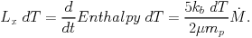
the gas density squared. For the part of the plasma that is steadily
cooling to lower temperature, each temperature interval has to
contribute to the cooling radiation with a power equal to the enthalpy
change of the plasma that is cooling across this temperature interval:
, as sketched in
Fig. 21. This simplified
picture of a reservoir of hot gas and a constant fraction of gas cooling
is motivated by the fact that cooling is accelerating with decreasing
temperature because the plasma is getting denser while it is cooling in
pressure equilibrium and the cooling radiation power is proportional to
the gas density squared. For the part of the plasma that is steadily
cooling to lower temperature, each temperature interval has to
contribute to the cooling radiation with a power equal to the enthalpy
change of the plasma that is cooling across this temperature interval:
 |
(11) |
To calculate the expected spectrum we have to weight this power by the ratio of the emission at a certain frequency to the bolometric emission:
 |
(12) |
To obtain the total spectrum radiated by all steady cooling temperature phases we have to integrate the above equation over dT:
 |
(13) |
where 
 (T) and
bol(T) are the emissivity of the
plasma (radiation power per unit emission measure) for radiation at
frequency, , and for
bolometric radiation, respectively.
(T) and
bol(T) are the emissivity of the
plasma (radiation power per unit emission measure) for radiation at
frequency, , and for
bolometric radiation, respectively.
With the advent of high quality spectra provided by XMM-Newton and Chandra, the cooling flow paradigm could be tested by spectroscopy. First evidence that the cluster cool cores are not consistent with the classical cooling flow model came from spectra analyzed with the Reflection Grating Spectrometers on XMM-Newton. Some of the cool core clusters have such highly peaked surface brightness profiles, that they look almost like blurred point sources to the RGS (which operates analogously to slitless spectroscopy in optical astronomy). Therefore the RGS can obtain spectra with much higher resolution than provided by the imaging CCD devices of the XMM-Newton EPIC cameras for these very peaked cool core regions. Fig. 22 shows the first published RGS spectrum of one of the very strong cool core clusters, A1835, at a redshift of z = 0.2523 (Peterson et al. 2001). In the Figure the observed XMM-Newton spectrum (dark red) is compared to the prediction for the cooling flow model with a mass deposition rate inferred from the total radiative emission in the cooling flow region determined from the X-ray images (blue curve). There are clearly some expected lines, notably those of Fe XVII, missing in the observations. A more detailed analysis of the spectrum shows that for an ambient ICM temperature of 8.2 keV, the central regions shows temperature phases down to about 2.7 keV, but the expected intermediate temperature phases below 2.7 keV are absent in the spectrum. This was generally taken as the first evidence that there is something wrong with the classical cooling flow model. Since at the same time high angular resolution Chandra images showed signs of strong interaction of the central AGN with the ambient ICM in many cool core regions (e.g. David et al. 2001, Nulsen et al. 2002, Fabian et al. 2005), the most probable solution to the absence of strong cooling was soon believed to be the heating of cool core regions by the central AGN.
 |
Figure 22. XMM-Newton RGS spectrum of the central region of the prominent cool core cluster, A1835 compared to model predictions (Peterson et al. 2001). The red line shows a spectral model for an isothermal temperature of 8.2 keV. The blue line shows the expectation for the classical cooling flow and an ambient temperature of 8.2 keV, the green line shows a cooling flow model where temperatures below 2.7 keV have been truncated. Clearly, some of the cooling flow predicted lines are missing from the observed spectrum. |
The spectral signature of the absence of cooling was not only obtained
from XMM-Newton RGS spectra. For example for the cool core
region in the X-ray halo of M87, the central dominant galaxy in the
northern part of the Virgo cluster, clear evidence for an inconsistency
of the spectral signatures with a classical cooling flow model could
also be provided by results with the EPIC pn and MOS cameras of
XMM-Newton. The most prominent feature that can be used for
these diagnostics is the blend of Fe lines in the spectrum from
transitions into the L-shell at photon energies around 1 keV.
Fig. 23 shows how the spectral feature of this
blend of
Fe lines changes with temperature. The shift is caused by the changing
degree of ionization of the Fe ions that contribute to the line
blend. When the temperature is lowered more and more electrons in the Fe
ions shield the charge of the nucleus decreasing the binding energy of
the L-shell electrons. As illustrated in Fig. 23
this spectral feature can be used as a sensitive thermometer in the
temperature range of 0.2-2 keV
(Böhringer
et al. 2002).
The middle panel in Fig. 23 shows the spectrum
implied for the broad
temperature distribution expected for the cooling flow in M87 (in the
radial range 1-2 arcmin) with a mass deposition rate of
~ 1
M yr-1. The predicted spectrum is clearly
different from the observed one. A way to modify the predicted spectrum
in the direction of the observed one, is to assume that the central
region of M87 is highly absorbed by cold or warm material to
reduce the
low energy part of the broad Fe line feature. The actual absorption can
be determined directly, however, by using the power law spectrum of the
M87 AGN with the result that there is no significant
excess absorption
above the known value of the galactic absorption column density of about
1.8 × 1020 cm-2. A very good fit to the
observed spectrum is then obtained by assuming that the bulk of the
plasma in the central region of the M87 halo only occupies a narrow
temperature interval of about 1.44 to 2 keV
(Böhringer
et al. 2002)
as shown in the right panel of Fig. 23.
yr-1. The predicted spectrum is clearly
different from the observed one. A way to modify the predicted spectrum
in the direction of the observed one, is to assume that the central
region of M87 is highly absorbed by cold or warm material to
reduce the
low energy part of the broad Fe line feature. The actual absorption can
be determined directly, however, by using the power law spectrum of the
M87 AGN with the result that there is no significant
excess absorption
above the known value of the galactic absorption column density of about
1.8 × 1020 cm-2. A very good fit to the
observed spectrum is then obtained by assuming that the bulk of the
plasma in the central region of the M87 halo only occupies a narrow
temperature interval of about 1.44 to 2 keV
(Böhringer
et al. 2002)
as shown in the right panel of Fig. 23.
 |
 |
 |
Figure 23. Left: Spectrum
of hot plasma at various temperatures around the Fe L-shell line blend
near 1 keV as observed with the response function of the
XMM-Newton EPIC pn instrument. This feature lends itself as a
nice thermometer for the temperature range 0.2 to 2 keV. Middle:
Predicted X-ray spectrum around the Fe L-shell line blend for the
cooling flow in the X-ray halo of M87 with a mass deposition rate of
|
||
It has to be noted that the interpretation of spectra from cooling flows had an interesting history already before the launch of Chandra and XMM-Newton. For example Ikebe et al. (1997) and Makishima (1999) already argued on the basis of ASCA spectroscopy with similar arguments as those given above for M87, that the prediction of cooling flow models is not met by the observations. The counterargument to keep the cooling flow model alive at the time was to postulate internal absorption (see e.g. Allen et al. 2001). The spectral resolution and sensitivity of ASCA was not quite good enough, however, to reject the cooling flow model in the very compelling way as now done with the XMM-Newton results. Even earlier, spectroscopic analysis of the X-ray halo of M87 with the Crystal Spectrometer on board of the Einstein satellite showed the emission lines for the cool phases expected in cooling flows Canizares et al. 1979, 1982), that we are now missing in modern observations. This evidence for steady state cooling in cooling flows gave actually one of the strongest supports to the cooling flow scenario at the time. It is now clear, however, that the results obtained in these early days were most probably features of spectral noise.
Deep observations of cool core regions, in particular with the XMM-Newton RGS instrument, have now also been used to characterize the multi-temperature structure in cool cores in more detail in terms of the emission measure (or luminosity) distribution of the plasma as a function of temperature (e.g. Peterson et al. 2003, Kaastra et al. 2004). This works well only in colder systems. Fig. 24 shows in the left panel the differential emission measure distribution in the cool core region of the cluster Abell 262 in the innermost four shells out to 3 arcmin. These observations can be compared to the expected emission measure distribution for the model of an isobaric cooling flow, shown in the middle panel of Fig. 24 (Kaastra et al. 2004). While the temperature distribution is not isothermal, we clearly note that the emission measure distribution falls off much more steeply than the model expectations towards lower temperatures, highlighting again the fact that less plasma is observed at lower temperatures than required for the cooling flow model. A similar result is shown - in the right panel of the Figure - for the case of the Centaurus cluster taken from Sanders et al. (2008) based on a very deep XMM-Newton observations of the cluster with the RGS instruments as well as deep Chandra data. Here we can follow the local temperature distribution of the plasma over a full decade in temperatures from about 0.4 to 4 keV. But again the contribution of the very low temperature phases is much less than what is expected for unimpeded cooling.
 |
 |
 |
Figure 24. Left: Differential
emission measure distribution as a function
of temperature of the plasma in the cool core region of the cluster
Abell 262 as deduced from a spectral analysis of
XMM-Newton
RGS observations. The results are derived for the innermost four
shells: 0 - 0.5 armin (triangles), 0.5 - 1 armin (squares), 1 - 2
arcmin (stars), 2-3 arcmin (circles). For comparison the dashed line
shows an approximation to the slope of the isobaric cooling flow model
(Kaastra et
al. 2004).
Middle: Differential emission measure distribution for the isobaric
cooling flow model, for 0.5 solar abundance
(Kaastra et
al. 2004)
Right: Differential emission measure distribution of the plasma
in the inner 2 arcmin region in the core of the Centaurus cluster of
galaxies. The results from a spectral analysis of XMM-Newton
RGS and CHADRA are shown for comparison. The solid line shows the
expected emission measure distribution for a 10
M |
||
As the change from the cooling flow paradigm to an AGN feedback scenario seems to be now widely accepted, the interest has shifted to the question: how is the ICM actually heated by AGN interaction? One of the most important earlier arguments in favour of cooling flows in the absence of feedback was that any possible heating mechanism has to be very well fine tuned, to exactly provide the balance to cooling. If too much heat is produced, it disperses the observed dense gas cores in cooling flows. Secondly, we observe increasing entropy profiles in the ICM of clusters (Fig. 13). It therefore has to be explained how central heating can work without inverting the entropy profiles leading to the dissipation of heat by convection. Both requirements need to be met and seem almost improbable (Fabian 1994). This makes it even more interesting now to understand how nature achieves this fine tuning.
One of the first, best studied cases is that of the Perseus cluster, which has now been observed with the Chandra observatory for more than 1 Million seconds as proposed by Fabian et al. (2005) providing the most detailed picture of a central cool core region. Fig. 25 shows a multi-colour image of the central region of the Perseus cluster from Fabian et al. (2005). The "false colour" image was produced from images in three energy bands 0.3-1.2 keV, 1.2-2 keV, and 2-7 keV. An image smoothed on a scale of 10 arcsec (with 80% normalization) has been subtracted from the image to highlight regions of strong density contrast. The central, bright part of the image shows two features of low surface brightness, interpreted as two cavities of the X-ray emitting plasma filled with the relativistic plasma from the radio jets of the central AGN. This region is surrounded by a series of nearly concentric "ripples" which are more clearly brought out by the unsharp masking processing of the image.
 |
Figure 25. False colour image of the central region of the Perseus cluster produced from images in three energy bands 0.3-1.2 keV, 1.2-2 keV, and 2-7 keV. An image smoothed on a scale of 10 arcsec (with 80% normalization) has been subtracted from the image to highlight regions of strong density contrast. The image shows a series of nearly concentric "ripples" which are interpreted as sound waves or weak shock waves set off by the activity of the central AGN (Fabian et al. 2006). |
A more detailed analysis of the density and temperature variations across the ripples, shown in Fig. 26, implies typical pressure variations associated with the ripples with amplitudes of about ± 5-10%, which are interpreted as sound waves or very weak shock waves in the innermost region. As detailed in Fabian et al. (2005) the dissipation of the sound waves - if the viscosity is sufficiently high - can balance the radiative cooling in the cool core by heating with the realistic assumption that the sound waves cross the cool core region in about 1/50 of the cooling time.
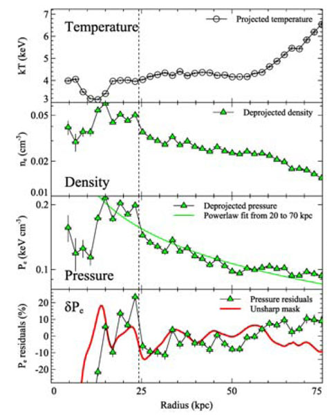 |
Figure 26. Temperature, density, pressure, and pressure residual profiles in the core region ICM of the Perseus cluster in a sector to the North-East (Fabian et al. 2006). The red line shows the ripples from an unsharp mask image. The dashed line marks the position of a shock front. |
Fabian et
al. (2006)
have also carried out multi-temperature plasma modeling in
various regions of the cluster centre and produced mass distribution maps
of plasma at temperatures around 0.5, 1, 2 and 4 keV. These maps are
shown in comparison to a map of the optical
H emission (observed by
Conselice et
al. 2001)
in Fig. 27. The distribution of the lowest
temperature phase around 0.5 keV has a striking similarity
to the H map. There is
relatively little plasma at 1 keV, mostly
in the very center of the cool core. The 2 keV phase coincides mostly
with the denser regions of the ICM. This detailed picture of the central
region of the Perseus cluster given in a series
of papers by Fabian et al. and Sanders et al. well illustrate the
frontier of the application of X-ray spectroscopy and thermodynamic
analysis of the ICM in the bright central regions of clusters.
emission (observed by
Conselice et
al. 2001)
in Fig. 27. The distribution of the lowest
temperature phase around 0.5 keV has a striking similarity
to the H map. There is
relatively little plasma at 1 keV, mostly
in the very center of the cool core. The 2 keV phase coincides mostly
with the denser regions of the ICM. This detailed picture of the central
region of the Perseus cluster given in a series
of papers by Fabian et al. and Sanders et al. well illustrate the
frontier of the application of X-ray spectroscopy and thermodynamic
analysis of the ICM in the bright central regions of clusters.
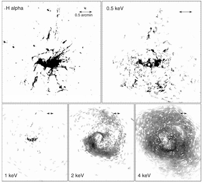 |
Figure 27.
H |
To show that the physics of the cool core regions seems to be quite diverse and that we can obviously not easily generalize the behaviour of the Perseus cluster to all cool core clusters we show two further examples of systems studied in detail, that of M87 and of Hydra A. M87 was studied in very much detail by a combination of a 500 ks exposure with Chandra (Forman et al. 2005, 2007) and a 120 ks exposure with XMM-Newton (Simionescu et al. 2007, 2008b). The X-ray halo of M87 is the closest of all cool core regions in galaxy clusters and can therefore be studied at the highest spatial resolution. Also the AGN in the center of M87 is active and is interacting with the ambient ICM through relativistic jets (e.g. Böhringer et al. 1995, Churazov et al. 2001). The deep Chandra exposure shows a surface brightness discontinuity which can be almost followed over the entire circumference of a ring around the nucleus with a radius of 14 kpc (Fig. 28, Forman et al. 2005, 2007). Another arc-shaped discontinuity is seen over a smaller sector region at the radius of 17 kpc. These features are identified as shock waves in Forman et al. (2005) and Forman et al. (2007). A detailed spectroscopic analysis of the M87 X-ray halo with XMM-Newton can corroborate this interpretation and give enhanced physical constraints. While the density discontinuity seen with Chandra implies a shock Mach number of about 1.2, the temperature jump seen in the projected spectra is about 5% at about 2 keV and implies a shock Mach number of > 1.05 without deprojection correction (Simionescu et al. 2007). Thus the temperature enhancement identifies the surface brightness discontinuity definitely as a weak shock front. The shock front has also been visualized in a pressure map of the M87 halo constructed from the XMM-Newton data shown in Fig. 28 (Simionescu et al. 2007). Similar to the hydrodynamic maps described above this map has been derived from spectral modeling in many spatial pixel, which in this case have been constructed by means of a Voronoi tessellation technique developed by Diehl & Statler (2006) and originally by Cappellari & Copin (2003) such that each pixel has a spectral signal to noise of at least 100. To enhance the visibility of discontinuities in the presence of the strong pressure gradient, a smooth, spherically symmetric model has been subtracted from the pressure distribution shown in Fig. 28. The map clearly shows a pressure enhancement at the shock radius of 3' (14 kpc) which implies without projection correction a Mach number larger than 1.08. There are some further interesting features seen in the pressure map. Outside the shock front we note two regions of lower pressure in the NE and in the SW. These are the regions where radio lobes filled with relativistic plasma emerging from the central AGN are observed. This observation thus implies that (at least part of) the missing pressure in these regions comes from the pressure of the relativistic plasma in the lobes, which does not contribute to the X-ray emission analysed here. Further insight into the physics of this interesting cool core region in M87 will be described in connection with the analysis of the element abundance distribution discussed in the next section.
 |
 |
Figure 28. Left: Chandra image of the X-ray halo of M87 in the 0.5-2.5 keV band (Forman et al. 2005). Several features are marked on this image: the surface brightness enhancements coinciding with the radio lobes (SW arm and E arm) and several sharp surface brightness discontinuities (14 kpc ring, 17 kpc arc, and 37 kpc arc) which are identified as shock fronts. Right: Map of the pressure deviations from a smooth spherical symmetric model derived from a deep XMM-Newton observation of the M87 halo (Simionescu et al. 2007). The 14 kpc ring is now clearly revealed as a pressure discontinuity supporting the shock interpretation. The regions of the radio lobes (SW arm and E arm) are now showing up as zones of pressure deficit, which is probably compensated for by the unseen pressure of the relativistic radio plasma. |
|
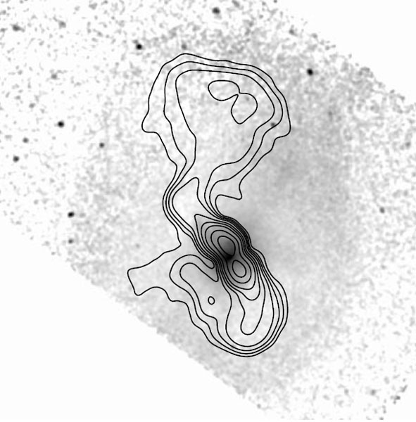
In a combined Chandra and XMM-Newton study of the central region of the galaxy cluster associated with the radio source Hydra A, a similar front diagnostics has also been performed by Nulsen et al. (2005) and Simionescu et al. (2008a). Here the shock feature has a radial extent of 200 - 300 kpc and hints at an event which was much more powerful by about two orders of magnitude than that in M87. Fig. 29 shows again the surface brightness discontinuity clearly detected in the high angular resolution image obtained with the Chandra observatory (Nulsen et al. 2005). A deep XMM-Newton observation then provides higher photon statistics that allows us to study this discontinuity spectroscopically. Firstly, we can again visualize the shock front as a pressure jump in the XMM-Newton based pressure map shown in Fig. 29 (Simionescu et al. 2008a). A more detailed analysis of the temperature and density distribution around the shock front in several sectors, shown in Fig. 30, provides more detailed information about the shock strength. Modeling the discontinuity in three dimensions and fitting the projected model to the data implies a Mach number of the best fitting model of about 1.2-1.3 (Simionescu et al. 2008a). Simple one-dimensional modeling of the evolution of the shock driven by the energy input of the radio lobes as well as detailed three-dimensional hydrodynamical simulations provide good estimates for the age and the total energy of the event causing the shock wave, with values for the age of ~ 2 × 10⁷ yr and the energy of 1061 erg (Nulsen et al. 2005, Simionescu et al. 2008a).
 |
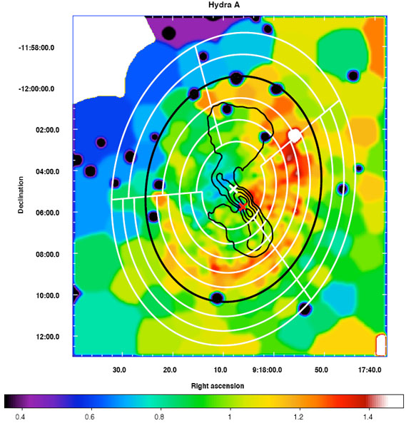 |
Figure 29. Left: Chandra image of Hydra A with the radio lobes superposed (Nulsen et al. 2005). An oval shaped surface brightness discontinuity at a radius of about 200 - 300 kpc can be noted that is identified with a shock wave caused by an energetic radio jet outburst. Right: Map of the pressure deviations from a smooth azimuthally symmetric model derived from a deep XMM-Newton observation of Hydra A (Simionescu et al. 2008a). The location of the X-ray surface brightness discontinuity observed in the Chandra image is approximated by the elliptical black line. A clear pressure jump can be seen almost all along this line indicating a shock front with a Mach number of about 1.3. |
|
 |
 |
Figure 30. Left: Model of the effect of a shock front with different Mach numbers predicting the observed surface brightness distribution in the XMM-Newton image of Hydra A (Simionescu et al. 2008a) Right: Temperature profile around the shock front compared to a smooth model (blue lines). The observed temperature and density (surface brightness) jumps are consistent with a shock wave with Mach number ~ 1.3 (Simionescu et al. 2008a). |
|
These few examples show the complex and probably very diverse physics prevailing in cluster cool core regions. We hope that further detailed studies of a larger sample of cool core regions will help to generalize the scenario of cool core heating. A major break through is also expected here from future high resolution spectroscopy, which will allow us to observe turbulent and bulk motions in the ICM as described in section 7.