


We are now at the point where we can discuss why molecular clouds collapse to form stars, and explore the basic physics of that collapse. We will first look at instabilities that cause collapse, and then discuss what happens when collapse occurs.
In considering whether molecular clouds can collapse, it is helpful to
look at the virial theorem, equation (85).
We can group the terms on the right hand side into those that are
generally or always positive, and thus oppose collapse, and those that
are generally or always negative, and thus encourage it. The main terms
opposing collapse are  ,
which contains parts describing both thermal pressure and turbulent
motion, and
,
which contains parts describing both thermal pressure and turbulent
motion, and  , which
describes magnetic pressure and tension. The main terms favoring
collapse are
, which
describes magnetic pressure and tension. The main terms favoring
collapse are  , representing
self-gravity, and
s, representing
surface pressure. The final term, the surface one, could be positive or
negative depending on whether mass is flowing into our out of the virial
volume. We will begin by examining the balance among these terms, and
the forces they represent.
, representing
self-gravity, and
s, representing
surface pressure. The final term, the surface one, could be positive or
negative depending on whether mass is flowing into our out of the virial
volume. We will begin by examining the balance among these terms, and
the forces they represent.
4.1.1. Thermal Pressure: the Bonnor-Ebert Mass
To begin with, consider a cloud where magnetic forces are negligible, so
we need only consider pressure and gravity. For simplicity we'll adopt a
spherical geometry, since more complex geometries only change the result
by factors of order unity, and we will neglect the flux of mass across
the cloud surface, since on average that contributes neither to support
nor to collapse. Thus we have a spherical cloud of mass M and
radius R, bounded by an external medium that exerts a pressure
Ps at its surface. The material in the cloud has a
one-dimensional velocity dispersion
 (including thermal and
non-thermal motions). With this assumption, the terms that appear on the
right-hand side of the virial theorem are
(including thermal and
non-thermal motions). With this assumption, the terms that appear on the
right-hand side of the virial theorem are
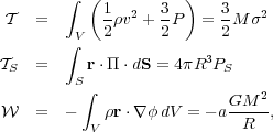 |
(93) (94) (95) |
where a is a constant of order unity that depends on the internal density distribution of the cloud.
If we wish the cloud to be in virial equilibrium, then we have
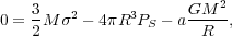 |
(96) |
which we can re-arrange to
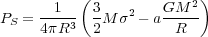 |
(97) |
This expression has an interesting feature. If we consider a cloud of
fixed M and and
vary the radius R, we find that Ps has a
maximum value
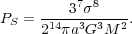 |
(98) |
We can understand what is going on physically as follows. Consider starting a cloud at very large radius R. In this case its self-gravity is negligible, so the second term in parentheses is can be dropped, but the mean density is very low and so the pressure is low. As we decrease the radius the pressure rises initially, but as the radius gets larger self-gravity starts to become important, and more and more of the cloud's internal pressure goes to holding it up against self-gravity, rather than against the external surface pressure. Eventually we reach a point where further contraction is counter-productive and actually lowers the surface pressure.
Now turn this around: if we consider a cloud with a fixed mass and internal velocity dispersion, and we vary the surface pressure, this means that, once the pressure exceeds a fixed value, there is no way that the cloud can remain in virial equilibrium. Instead, it must collapse. The maximum possible pressure is a decreasing function of mass, so larger and larger masses become progressively more and more unstable.
In order to be more quantitative about this, we need to know the value of a, which depends on the internal density distribution. We can solve for this by writing down the equation of hydrostatic balance for the cloud and finding the value of a from the self-consistently determined density distribution. We won't do so in these notes, but the result can be found in standard textbooks. The result is that the maximum mass that can be held up in an environment where the surface pressure is Ps is
 |
(99) |
This is known as the Bonnor-Ebert mass. The scalings chosen for
and
Ps are typical of the thermal sound speed and the
pressure in molecular clouds, and it is certainly interesting that when
we plug in these values we get something like the typical mass of a
star.
Of course if we put in the typical observed velocity dispersion in
molecular clouds, ~ a
few km s-1, we get a vastly larger mass - more like
104 - 106
M , the
mass of a GMC. This makes sense. It's equivalent to our statement from
above that the virial ratios of molecular clouds are about
unity. However, turbulent support is a tricky thing. It doesn't work
everywhere. In some places the turbulent flows come together and cancel
out, and in those places the velocity dispersion drops to the thermal
value, and collapse can occur if the mass exceeds the Bonnor-Ebert
mass. We'll return to this idea of large-scale support by turbulence
coupled with localized collapse in the final section.
, the
mass of a GMC. This makes sense. It's equivalent to our statement from
above that the virial ratios of molecular clouds are about
unity. However, turbulent support is a tricky thing. It doesn't work
everywhere. In some places the turbulent flows come together and cancel
out, and in those places the velocity dispersion drops to the thermal
value, and collapse can occur if the mass exceeds the Bonnor-Ebert
mass. We'll return to this idea of large-scale support by turbulence
coupled with localized collapse in the final section.
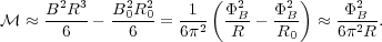
4.1.2. Magnetic Support: the Magnetic Critical Mass
Now let us consider a cloud where the magnetic term in the virial theorem greatly exceeds the kinetic one. Again, we'll consider a simple case to get the basic scalings: a uniform spherical cloud of radius R threaded by a magnetic field B. We imagine that B is uniform inside the cloud, but that outside the cloud the field lines quickly spread out, so that the magnetic field drops down to some background strength B0, which is also uniform but has a magnitude much smaller than B.
The magnetic term in the virial theorem is
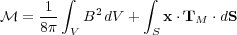 |
(100) |
where
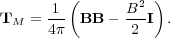 |
(101) |
If the field inside the cloud is much larger than the field outside it, then the first term, representing the integral of the magnetic pressure within the cloud, is
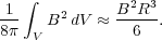 |
(102) |
Here we have dropped any contribution from the field outside the cloud. The second term, representing the surface magnetic pressure and tension, is
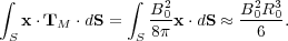 |
(103) |
Since the field lines that pass through the cloud must also pass through
the virial surface, it is convenient to rewrite everything in terms of
the magnetic flux. The flux passing through the cloud is
 B =
B =
 B R2,
and since these field lines must also pass through the virial surface,
we must have B
= B0
R02 as well. Thus, we can rewrite the
magnetic term in the virial theorem as
B R2,
and since these field lines must also pass through the virial surface,
we must have B
= B0
R02 as well. Thus, we can rewrite the
magnetic term in the virial theorem as
 |
(104) |
In the last step we used the fact that R << R0 to drop the 1 / R0 term.
Now let us compare this to the gravitational term, which is
 |
(105) |
for a uniform cloud of mass M. Comparing these two terms, we find that
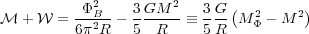 |
(106) |
where
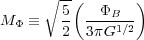 |
(107) |
We call
M
the magnetic critical mass.
Since both B
does not change as a cloud expands or contracts (due to flux-freezing),
this magnetic critical mass does not change either. The implication of
this is that clouds that have M >
M always have
+
< 0. The magnetic
force is unable to halt collapse no matter what. Clouds that satisfy
this condition are called magnetically supercritical, because they are
above the magnetic critical mass
M. Conversely, if M <
M, then +
> 0, and gravity is
weaker than magnetism.
Clouds satisfying this condition are called subcritical. For a
subcritical cloud, since +
 1 / R, this
term will get larger and larger as the cloud shrinks. In other words,
not only is the magnetic force resisting collapse is stronger than
gravity, it becomes larger and larger without limit as the cloud is
compressed to a smaller radius. Unless the external pressure is also
able to increase without limit, which is unphysical, then there is no
way to make a magnetically subcritical cloud collapse. It will always
stabilize at some finite radius. The only way to get around this is to
change the magnetic critical mass, which requires changing the magnetic
flux through the cloud. This is possible only via ambipolar diffusion or
some other non-ideal MHD effect that violates flux-freezing.
1 / R, this
term will get larger and larger as the cloud shrinks. In other words,
not only is the magnetic force resisting collapse is stronger than
gravity, it becomes larger and larger without limit as the cloud is
compressed to a smaller radius. Unless the external pressure is also
able to increase without limit, which is unphysical, then there is no
way to make a magnetically subcritical cloud collapse. It will always
stabilize at some finite radius. The only way to get around this is to
change the magnetic critical mass, which requires changing the magnetic
flux through the cloud. This is possible only via ambipolar diffusion or
some other non-ideal MHD effect that violates flux-freezing.
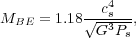
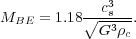
Of course our calculation is for a somewhat artificial configuration of a spherical cloud with a uniform magnetic field. In reality a magnetically-supported cloud will not be spherical, since the field only supports it in some directions, and the field will not be uniform, since gravity will always bend it some amount. Figuring out the magnetic critical mass in that case requires solving for the cloud structure numerically. A calculation of this effect by Tomisaka et al. [17] gives
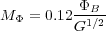 |
(108) |
for clouds for which pressure support is negligible. The numerical coefficient we got for the uniform cloud case is 0.17, so this is obviously a small correction. It is also possible to derive a combined critical mass that incorporates both the flux and the sound speed, and which limits to the Bonnor-Ebert mass for negligible field and the magnetic critical mass for negligible pressure.
Given that a sufficiently strong magnetic field can prevent the collapse of a cloud, it is a critical question whether molecular clouds are super- or subcritical. This must be answered empirically. Observations of magnetic fields in molecular clouds are extremely difficult, and we will not take the time to go into the various techniques that are used. Nonetheless, the observations at this point do seem to show that molecular clouds are magnetically supercritical, although not by a lot - see Figure 4. However, since this is a difficult observation, this interpretation of the data is not universally accepted.
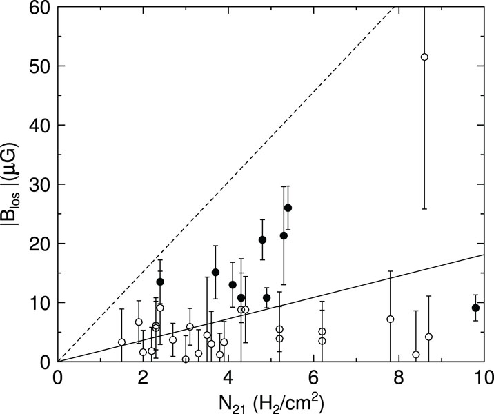 |
Figure 4. Measurements of the line of sight
magnetic field strength Blos in a sample of molecular
cloud cores, as a function of the number density of H2
molecules N21 (in units of 1021 molecules
cm-2). Filled points show detections, while empty points
show upper limits. The dashed line is the division between magnetically
subcritical (above the line) and magnetically supercritical (below the
line). Error bars are
1 |
The simplest case to think about, and a good one to understand some of the basic physical processes, is the collapse of a non-rotating, non-turbulent, isothermal spherical core without a magnetic field, supported by thermal pressure. Of course none of these assumptions are strictly true, but they give us a place to begin our study. Moreover, the assumption that collapsing regions, called cores, are not strongly supersonic is reasonable, since collapse tends to occur in places where the turbulent velocities cancel. Observations show this, e.g. as illustrated in Figure 5.
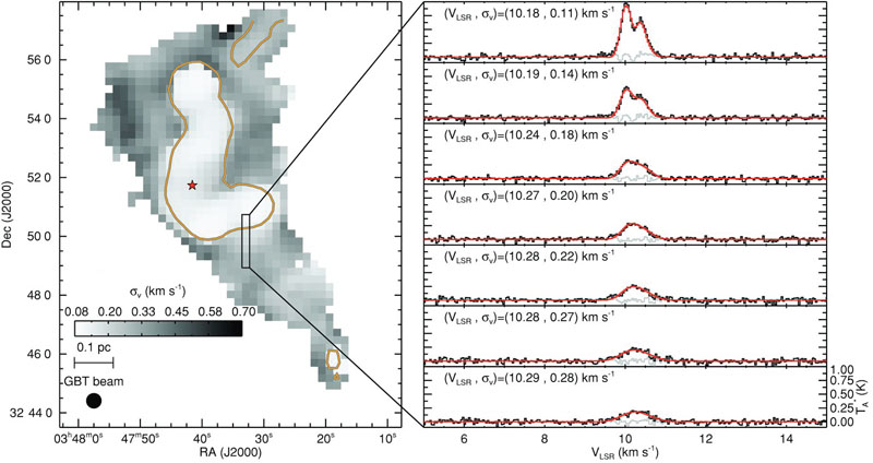 |
Figure 5. Measurements of the velocity dispersion of the gas in and around a dense core, measured using ammonia (NH3) lines. The grayscale image on the left shows the velocity dispersion as a function of position, and on the right the figure shows the measured spectra at the indicated positions. Reprinted with permission from the AAS from [19]. |
Density and Velocity Profiles
Consider a sphere of gas with an initial density distribution
 (r).
We would like to know how the gas moves under the influence of gravity
and thermal pressure, under the assumption of spherical symmetry. For
convenience we define the enclosed mass
(r).
We would like to know how the gas moves under the influence of gravity
and thermal pressure, under the assumption of spherical symmetry. For
convenience we define the enclosed mass
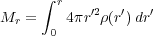 |
(109) |
or equivalently
 |
(110) |
The equation of mass conservation for the gas in spherical coordinates is
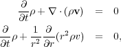 |
(111) (112) |
where v is the radial velocity of the gas.
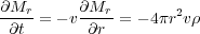
It is useful to write the equations in terms of Mr
rather than ,
so we take the time derivative of Mr to get
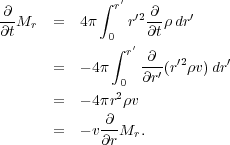 |
In the second step we used the mass conservation equation to substitute
for  t, and in the
final step we used the definition of Mr to substitute
for . To
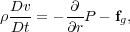
figure out how the gas moves, we write down the Navier-Stokes equation
without viscosity, which is just the Lagrangean version of the momentum
equation:
t, and in the
final step we used the definition of Mr to substitute
for . To
figure out how the gas moves, we write down the Navier-Stokes equation
without viscosity, which is just the Lagrangean version of the momentum
equation:
 |
(113) |
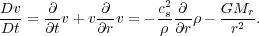
where fg is the gravitational force. For the momentum
equation, we take advantage of the fact that the gas is isothermal to
write P =
cs2. The gravitational force is
fg = -G Mr /
r2. Thus we have
 |
(114) |
For a given set of initial conditions, it is generally very easy to solve these equations numerically, and in some cases to solve them analytically. To get a sense of what to expect, let's think about the behavior in the limit of zero gas pressure, i.e. cs = 0. We take the gas to be at rest at t = 0. This is not as bad an approximation as you might think. Consider the virial theorem: the thermal pressure term is just proportional to the mass, since the gas sound speed stays about constant. On the other hand, the gravitational term varies as 1/R. Thus, even if pressure starts out competitive with gravity, as the core collapses the dominance of gravity will increase, and before too long the collapse will resemble a pressureless one.
In this case the momentum equation is trivial:
 |
(115) |
This just says that a shell's inward acceleration is equal to the gravitational force per unit mass exerted by all the mass interior to it, which is constant. We can then solve for the velocity as a function of position:
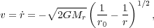 |
(116) |
where r0 is the position at which a particular fluid
element starts. To integrate again and solve for r, we make the
substitution r = r0
cos2 [20]:
[20]:
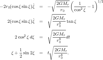 |
(117) (118) (119) (120) |
We are interested in the time at which a given fluid element reaches the
origin, r = 0. This corresponds to
=
/ 2, so this time is
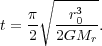 |
(121) |
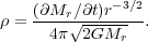
Suppose that the gas we started with was of uniform density
, so that
Mr =
(4/3)
r03
. In this
case we have
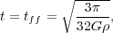 |
(122) |
where we have defined the free-fall time tff: it is the time required for a uniform sphere of pressureless gas to collapse to infinite density.
For a uniform fluid this means that the collapse is synchronized - all
the mass reaches the origin at the exact same time. A more realistic
case is for the initial state to have some level of central
concentration, so that the initial density rises inward. Let's take the
initial density profile to be
=
c
(r / rc)- , where
> 0 so the density
rises inward. The corresponding enclosed mass is
, where
> 0 so the density
rises inward. The corresponding enclosed mass is
 |
(123) |
Plugging this in, the collapse time is
 |
(124) |
Since > 0, this
means that the collapse time increases with initial radius
r0.
This illustrates one of the most basic features of a collapse, which will continue to hold even in the case where the pressure is non-zero. Collapse of centrally concentrated objects occurs inside-out, meaning that the inner parts collapse before the outer parts. Within the collapsing region near the star, the density profile also approaches a characteristic shape. If the radius of a given fluid element r is much smaller than its initial radius r0, then its velocity is roughly
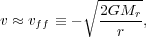 |
(125) |
where we have defined the free-fall velocity vff as the characteristic speed achieved by an object collapsing freely onto a mass Mr.
The mass conservation equation is
 |
(126) |
If we are near the star so that v
 vff, then this implies that
 |
(127) |
To the extent that we look at a short interval of time, over which the
accretion rate does not change much (so that
Mr
/ t is
roughly constant), this implies that the density near the star varies as
r-3/2.
The characteristic accretion rate
What sort of accretion rate do we expect from a collapse like this? For
a core of mass Mc = [4/(3 -
)]
c
rc3, the last mass element arrives at the
center at a time
 |
(128) |
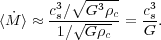
so the time-averaged accretion rate is
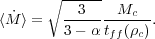 |
(129) |
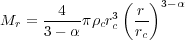
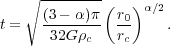
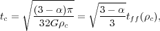
In order to get a sense of the numerical value of this, let us suppose that our collapsing object is a marginally unstable Bonnor-Ebert sphere, with mass
 |
(130) |
where Ps is the pressure at the surface of the sphere
and cs is the thermal sound speed in the core. Let's
suppose that the surface of the core, at radius rc, is
in thermal pressure balance with its surroundings. Thus
Ps =
c
cs2, so we may rewrite the Bonnor-Ebert mass as
 |
(131) |
A Bonnor-Ebert sphere doesn't have a powerlaw structure, but if we
substitute into our equation for the accretion rate and say that the
factor of [3/(3 -
)]1/2 is a
number of order unity, we find that the accretion rate is
 |
(132) |
This is an extremely useful expression, because we know the sound speed
cs from microphysics. Thus, we have calculated the
rough accretion rate we expect to be associated with the collapse of any
object that is marginally stable based on thermal pressure
support. Plugging in
cs = 0.2 km s-1, we get
 2 ×
10-6
M
yr-1 as the characteristic accretion rate for these objects.
2 ×
10-6
M
yr-1 as the characteristic accretion rate for these objects.
Since the typical stellar mass is a few tenths of
M, based
on the peak of the IMF, this means that the characteristic star
formation time is of order 105 - 106 yr. Of course
this conclusion about the accretion rate only applies to collapsing
objects that are supported mostly by thermal pressure. Other sources of
support produce higher accretion rates; this is typically the case for
massive stars.
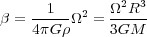
4.2.2. Rotation Collapse and the Angular Momentum Problem
The next element to add to this picture is rotation. We characterize the
importance of rotation through the ratio of rotational kinetic energy to
gravitational binding energy, which we denote
 . If the
angular velocity of the rotation is
. If the
angular velocity of the rotation is
 and the moment of
inertia of the core is I, this is
and the moment of
inertia of the core is I, this is
 |
(133) |
where a is our usual numerical factor that depends on the mass
distribution. For a sphere of uniform density
, we get
 |
(134) |
Thus we can estimate
simply
given the density of a core and its measured velocity gradient. Observed
values of
are typically a few percent
[21].
Let us consider how rotation affects the collapse, for a simple core of
constant angular velocity
. Consider a fluid
element that is initially at some distance r0 from the
axis of rotation. We will consider it to be in the equatorial plane,
since fluid elements at equal radius above the plane have less angular
momentum, and thus will fall into smaller radii. Its initial angular
momentum in the direction along the rotation axis is j =
r02
.
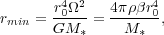
If pressure forces are insignificant for this fluid element, it will travel ballistically, and its specific angular momentum and energy will remain constant as it travels. At its closest approach to the central star plus disk, its radius is rmin and by conservation of energy its velocity is vmax = (2 G M* / rmin)1/2, where M* is the mass of the star plus the disk material interior to this fluid element's position. Conservation of angular momentum them implies that j = rmin vmax.
Combining these two equations for the two unknowns rmin and vmax, we have
 |
(135) |
where we have substituted in for
2 in
terms of .
This tells us the radius at which infalling material must go into a disk
because conservation of angular momentum and energy will not let it get
any closer.
We can equate the stellar mass M* with the
mass that started off interior to this fluid element's position - this
amounts to assuming that the collapse is perfectly inside-out, and that
the mass that collapses before this fluid element's all makes it onto
the star. If we make this approximation, then
M* = (4/3)
r03, and we get
 |
(136) |
i.e. the radius at which the fluid element settles into a disk is simply
proportional to
times a
numerical factor of order unity.
We shouldn't take the factor too seriously, since of course real clouds
aren't uniform spheres in solid body rotation, but the result that
rotation starts to influence collapse and force disk formation at a
radius that is a few percent of the core radius is interesting. It
implies that for cores that are ~ 0.1 pc in size and have
values
typical of what is observed, they should start to become rotationally
flattened at radii of several hundred AU. This will be the typical size
scale of protostellar disks.
In order for mass to actually get to a star, of course, its angular momentum must be redistributed outwards. It must get from hundreds of AU to << 1 AU. Fortunately, disks are devices whose sole purpose is to separate mass and angular momentum. We will not spend any more time on disks (which could form an entire lecture series of their own), except to say that they provide numerous possible mechanisms to remove the angular momentum from the bulk of the mass and allow it to reach the star.
4.2.3. Magnetized Collapse and the Magnetic Flux Problem
So far we have only dealt with pressure, rotation, and gravity. Now we will add magnetic fields to the picture. We will assume that we have a magnetically supercritical core, so that we need not worry about magnetic fields significantly inhibiting the collapse. Instead, we will work on a second problem: that of the magnetic flux.
As we discussed earlier, observed magnetic fields make cores marginally
supercritical, but only by factors of a few. If the collapse occurs in
the ideal-MHD regime, where perfect flux-freezing holds, then this mass
to flux ratio doesn't change. What sort of magnetic field would we then
expect stars to have? For the Sun, if we had
M
= M / 2, then we would expect the mean magnetic field to be
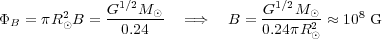 |
(137) |
For comparison, the observed mean surface magnetic field of the Sun is a few Gauss. Clearly this means that the Sun, and other stars like it, must have lost most of their magnetic fields during the collapse process. This means that the ideal MHD regime cannot apply, and resistivity or some other non-ideal effect must become significant.
There are two mechanisms which can lead to violation of flux-freezing in cores: ambipolar diffusion and Ohmic resistivity. As we saw in the last section, ambipolar diffusion will cause ions and neutrals to begin decoupling on scales below ~ 0.5 pc.
Decoupling does not prevent the field from increasing at all - there is always some inward drag exerted on the ions by the infalling neutrals, even if it is weak. This will eventually increase the field strength, which leads to the second effect: Ohmic resistivity. As the field lines are pressed closer together, field lines of opposite direction come into close proximity. When this happens, the field can reconnect, meaning that its topology changes and drops to a lower energy state. The excess energy is released in the form of heat. The microphysics of this process is not fully understood, but we see it happening in plasmas like the solar corona, where it is associated with flaring. Something similar must happen in protostellar cores in order to explain the observed low magnetic fields of stars.