


In this final section we'll come up to the present state of the art and talk about what are probably the two largest unsolved problems in star formation today: the star formation rate and the origin of the initial mass function.
5.1.1. The Observational Problem: Slow Star Formation
The problem of the star formation rate can be understood very simply. In the last lecture we computed the characteristic timescale for collapse to occur, and argued that, even if a collapsing region is only slightly unstable initially, this will not change the collapse time by much. Magnetic fields could delay or prevent collapse, but observations seem to indicate that they are not strong enough to do so. Thus we would expect that, on average, clouds will collapse on a timescale comparable to tff, and the rate of star formation in a galaxy should be the total mass of bound molecular clouds M divided by this.
To make this more concrete, we introduce the notation (first used by Krumholz & McKee [22])
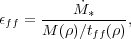 |
(138) |
where
M( )
is the gas mass in a given region with density
or larger,
tff is the free-fall time evaluated at that density,
and
)
is the gas mass in a given region with density
or larger,
tff is the free-fall time evaluated at that density,
and
 *
is the star formation rate in the region in question. The regions here
can be either entire galaxies are specified volumes within a galaxy. We
refer to
*
is the star formation rate in the region in question. The regions here
can be either entire galaxies are specified volumes within a galaxy. We
refer to  ff
as the dimensionless star formation rate or
star formation efficiency. Unfortunately the language here is somewhat
confused, because people sometimes mean something different by star
formation efficiency. To avoid confusion we will just use the symbol
ff.
ff
as the dimensionless star formation rate or
star formation efficiency. Unfortunately the language here is somewhat
confused, because people sometimes mean something different by star
formation efficiency. To avoid confusion we will just use the symbol
ff.
The argument we have just given suggests that
ff should
be of order unity if we pick
to be the
typical density of molecular clouds, or anything higher. However, the
actual value of
ff is
much smaller, as first pointed out by Zuckerman & Evans
[23].
The Milky Way's disk contains ~ 109
M of
GMCs inside the Solar circle
[24,
25],
and these have a mean density of n ~ 100 cm-3
[26],
corresponding to a free-fall time time tff
of
GMCs inside the Solar circle
[24,
25],
and these have a mean density of n ~ 100 cm-3
[26],
corresponding to a free-fall time time tff
 4 Myr. Thus
M / tff
250
M
yr-1. The observed star formation rate in the Milky Way is ~
1 M
yr-1
[27,
28].
Thus ff ~
0.01! Clearly our naive estimate is wrong.
4 Myr. Thus
M / tff
250
M
yr-1. The observed star formation rate in the Milky Way is ~
1 M
yr-1
[27,
28].
Thus ff ~
0.01! Clearly our naive estimate is wrong.
One can repeat this exercise in many galaxies and using many different
density tracers. One way is to measure the mass using a molecular tracer
with a known critical density, which effectively gives
M(),
compute tff() at that critical density, and compare to the
star formation rate. Krumholz & Tan
[29]
compiled the data available at the time and found that, for every tracer
for which they could make a measurement, and in every galaxy,
ff was
still ~ 0.01 (Figure 6). Subsequent more
accurate measurements in several large surveys, most notably the c2d
survey
[30],
give the same result. Thus, we have a problem: why is the star formation
rate about 1% of the naively estimated value?
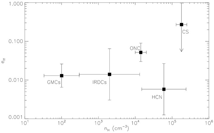 |
Figure 6. Observed star formation
efficiency per free-fall time
|
As a side note, the famous Kennicutt relation
[31],
which is an observed correlation between the star formation rate in a
given portion of a galaxy disk and the gas surface density in that
region. The observed normalization of the Kennicutt relation is
equivalent to the statement
ff ~ 0.01.
There are two major classes of proposed solution to this problem. One is the idea that molecular clouds aren't really gravitationally bound, and the other is the idea that clouds are bound, but that turbulence inhibits large-scale collapse while permitting small amount of mass to collapse.
Unbound GMCs
The unbound GMC idea is that most of the mass in molecular clouds is in
a diffuse state that is either not gravitationally bound, or that is
supported against collapse by strong magnetic fields. (The latter is not
ruled out because it is not easy to measure the magnetic field in very
diffuse molecular gas.) This idea would definitely work, in the sense
that it would produce low star formation rates, if GMCs really were
unbound. The main problem is that there is no observational evidence
that this is the case, and considerable evidence that it is not. In
particular, while we have no trouble finding low mass CO-emitting clouds
with virial ratios
 vir >>
1, CO-emitting clouds with masses
vir >>
1, CO-emitting clouds with masses
 104
M and
vir >>
1 do not appear to exist
[32].
If GMCs were really unbound, why do they all have virial ratios ~ 1?
104
M and
vir >>
1 do not appear to exist
[32].
If GMCs were really unbound, why do they all have virial ratios ~ 1?
A second problem with this idea is that, as we have seen
ff is ~
1% across of huge range of densities and environments. It is not at all
obvious why the fraction of mass that is bound would be the same at all
densities and across all galactic environments, from low-mass dwarfs to
massive ultraluminous infrared galaxies. The universality of the ~ 1%
seems to demand an explanation that is rooted in something more
universal than an appeal to fractions of a GMC that are bound versus
unbound.
Turbulence-Regulated Star Formation A more promising idea, which is probably the most generally accepted at this point (though it still has significant problems) is that the ubiquitous turbulence observed in GMCs serves to keep the star formation rate within them low. The first quantitative model of this in the hydrodynamic case was proposed by Krumholz & McKee [22], and it has since been extended to the MHD case by Padoan & Nordlund [33].
The basic idea of this model relies on two properties of supersonic
turbulence. Due to time limitations we will not prove these, but they
can be understood analytically, and the are reproduced in every
simulation. The first property is that turbulence obeys what is known as
a linewidth-size relation. This means that, if we consider a region of
size  and compute the
non-thermal velocity dispersion
and compute the
non-thermal velocity dispersion
 nt within it,
the velocity dispersion will depend on
. For subsonic turbulence
the relationship is
nt
nt within it,
the velocity dispersion will depend on
. For subsonic turbulence
the relationship is
nt
 1/3, while for
highly supersonic turbulence it is
1/2. This
relationship is in fact observed in molecular clouds.
1/3, while for
highly supersonic turbulence it is
1/2. This
relationship is in fact observed in molecular clouds.
Now consider the implications of this result in the virial theorem. On
large scales we know that clouds have
vir ~ 1, so
that | | ~
| ~
 . If we consider a random
region within a cloud of size
< R, where
R is the cloud radius, then the mass within that region will scale as
3, so the
gravitational potential energy will scale
as
M2 /
5. In comparison,
the kinetic energy varies as
M 2
4, since
2
for large
. Thus we expect that, for
an average region
. If we consider a random
region within a cloud of size
< R, where
R is the cloud radius, then the mass within that region will scale as
3, so the
gravitational potential energy will scale
as
M2 /
5. In comparison,
the kinetic energy varies as
M 2
4, since
2
for large
. Thus we expect that, for
an average region
 |
(139) |
Since
vir(R)
1, this means that
vir >>
1 for l << R, i.e. the typical, randomly chosen
region within a GMC is gravitationally unbound by a large margin. This
is in good agreement with observations: GMCs are bound, but random
sub-regions within them are not.
We can turn this around by asking how much denser than average a region
must be in order to be bound. For convenience we define the sonic length
as the choice of length scale
for which the non-thermal
velocity dispersion is equal to the thermal sound speed, i.e.
 |
(140) |
Now consider a region within a cloud with density
, chosen
small enough that the velocity dispersion is dominated by thermal rather
than non-thermal motions. The maximum mass that can be supported against
collapse by thermal pressure is the Bonnor-Ebert mass. If we let
be the
density at the surface of our Bonnor-Ebert sphere and we adopt a uniform
sound speed cs, then
= cs,
Ps =
cs2, and
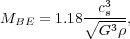 |
(141) |
and the corresponding radius of the maximum mass sphere is
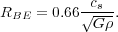 |
(142) |
We can compute the gravitational potential energy and the thermal energy of such a sphere from its self-consistently determined density distribution. The result is
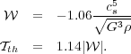 |
(143) (144) |
Similarly, we can compute the turbulent energy from the linewidth-size
relation evaluated at = 2
RBE. Doing so we have
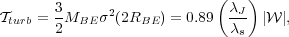 |
(145) |
where  j
= (
j
= ( cs2 /
G
)1/2
is called the Jeans length; it is just 2.7 times RBE.
cs2 /
G
)1/2
is called the Jeans length; it is just 2.7 times RBE.
This is a very interesting result. It says that the turbulent energy in
a maximal-mass Bonnor Ebert sphere is comparable to its gravitational
potential energy if the Jeans length is comparable to the sonic
length. Since the Jeans length goes up as the density goes down, this
means that, at low density,
turb >>
||, while at high density
turb >>
||. In order for a region
to be unstable to collapse, the latter condition must hold. We have
therefore identified a minimum density at which we expect sub-regions of
a molecular cloud to be unstable to collapse.
To get a sense of what this density is, let us evaluate
j /
s at the
mean density of a 104
M, 6
pc-sized molecular cloud. If such a cloud has
vir = 1, the
velocity dispersion at the cloud scale is
= 1.2 km
s-1; since cs = 0.2 km s-1, we
have
s = 0.15
pc. At the mean density of the cloud,
= 7.5
× 10-22 g cm-3, and
j = 1.5
pc. Thus
j >>
s, and at
the mean density things are unbound by a large margin. To be dense
enough to be bound, the density has to be larger than the mean by a
factor of
(s /
j)2
100, so bound
structures are those with
8 ×
10-20 g cm-3, or n
3 ×
104 cm-3.
In order to go further we must know something about the internal density
distribution in molecular clouds. We now invoke the second property of
supersonic isothermal turbulence: it generates a distribution of
densities that is lognormal in form. Formally, the point probability
distribution function of the density, meaning the probability of
measuring a density
at a given
position, obeys
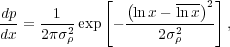 |
(146) |
where x =
/  is the
density divided by the volume-averaged density,
is the
density divided by the volume-averaged density,
 =
-2 / 2 is the mean of the logarithm of
the overdensity, and
is the
dispersion of log density. That the density distribution should be
lognormal isn't surprising. In a supersonically turbulent medium, each
shock that passes a point multiplies its density by a factor of the Mach
number of the shock squared, and each rarefaction front divides the
density by a similar factor. Thus the density at a point is a product of
many multiplications and divisions, and by the central limit theorem the
result of many such operations is a lognormal (just as the result of
doing many random additions and subtractions is a normal
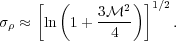
distribution). Empirical work shows that the width of the normal
distribution depends on the Mach number
=
-2 / 2 is the mean of the logarithm of
the overdensity, and
is the
dispersion of log density. That the density distribution should be
lognormal isn't surprising. In a supersonically turbulent medium, each
shock that passes a point multiplies its density by a factor of the Mach
number of the shock squared, and each rarefaction front divides the
density by a similar factor. Thus the density at a point is a product of
many multiplications and divisions, and by the central limit theorem the
result of many such operations is a lognormal (just as the result of
doing many random additions and subtractions is a normal
distribution). Empirical work shows that the width of the normal
distribution depends on the Mach number
 of the turbulence as
 |
(147) |
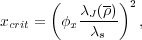
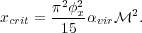
Now we can put together an estimate of the star formation rate. We
estimate that the gas that has a density larger than the critical
density given by the condition that
j <
s, which is
 |
(148) |
where  x is a factor of order unity. If we compute the
mean density and the sonic length for our fiducial cloud of mass
M, radius R, and velocity dispersion
, with a little algebra
we can show that
x is a factor of order unity. If we compute the
mean density and the sonic length for our fiducial cloud of mass
M, radius R, and velocity dispersion
, with a little algebra
we can show that
 |
(149) |
Gas above this density forms stars on a timescale given by the free-fall time at the mean density, since that is the timescale over which the density distribution will be regenerated to replace overdense regions that collapse to stars. Thus we have
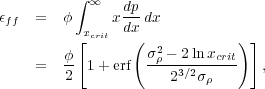 |
(150) (151) |
where
is another constant of order unity. Note that, except for the
factors,
everything in this expression is given in terms of
vir and
, i.e. in terms of the
virial ratio and Mach number of the cloud. The
factors can be
calibrated against simulations. For those who don't walk around with
graphs of the the error function in their heads (i.e. most of us),
it's useful to have a powerlaw approximation to this, which is
 |
(152) |
In other words, for a cloud with
~ 10-100 and
vir = 1, we
expect
ff ~
0.01, which nicely explains the observation that
ff ~ 0.01
everywhere. This analytic model also agrees well with numerical
simulations
[33].
Driving Turbulence This is a cute explanation, but it assumes that the turbulence is present and is capable of inhibiting star formation over the lifetime of a molecular cloud. This is not obvious, because we know from numerical experiments that turbulence decays quickly. This is not surprising. Every time there is a shock, kinetic energy is converted into thermal energy. Because radiative times are short compared to mechanical ones, as we showed earlier, all this energy is radiated away immediately, bringing the gas back to its original temperature. This represents a net loss of energy, and in the absence of a source to offset this loss the turbulence must decay. Numerical experiments show that the decay time is only about a crossing time of the cloud [14].
We therefore need an energy source to drive the turbulence. There are two main possibilities, both of which probably contribute. One is the gravitational potential energy released in the formation of the molecular cloud itself. As material falls onto the cloud it can drive turbulent motion, and as long as the cloud gains mass quickly from the larger ISM that is probably an important energy source [34, 35]. A second source, which is probably more important in evolved GMCs, is feedback from newly formed stars. Young stars produce strong jets that can drive motions in their parent clouds [36, 37], and they also produce ionizing radiation that can drive motions [38, 39]. Both of these effects can drive turbulence, and they probably dominates in more evolved clouds. Exactly what the energy balance in GMCs is, and how it is maintained, is not completely understood.
5.2. The Initial Mass Function
Our second unsolved problem in this lecture is the initial mass function (IMF). To begin, we have to define what the IMF means. It is simply the mass distribution of a population of stars at birth. We define this by a function
 |
(153) |
Note that dn / dm would be the number of stars per unit
mass, while
 (m) =
dn / d ln m = m (dn / dm) is the
mass of stars per unit mass, i.e.
(m) =
dn / d ln m = m (dn / dm) is the
mass of stars per unit mass, i.e.
 m1m2
(m)
dm is the fraction of the mass in a newborn stellar population
that is found in stars with masses between m1 and
m2.
m1m2
(m)
dm is the fraction of the mass in a newborn stellar population
that is found in stars with masses between m1 and
m2.
Observing the IMF is tricky, and there are three main approaches. One is to look at a young cluster and count the stars in it as a function of mass. This is the most straightforward approach, but it is limited by the number of young clusters where we can directly measure individual stars down to low masses. This means that we get a clean measurement, but the statistics are poor. A second approach is to rely on counts of field stars in the solar neighborhood that are no longer in clusters. Here the statistics are much better, but we can only use this technique for low mass stars, because for massive ones the number in the Solar neighborhood is determined more by star formation history than by the IMF. Finally, we can get limits on the IMF from the integrated light of a stellar populations.
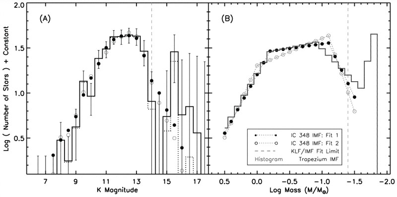 |
Figure 7. Measured K band luminosity functions (left) and stellar initial mass functions (right) for the cluster IC 348 (filled and open circles), and for the Trapezium cluster (histogram). Reprinted with permission from the AAS from [40]. |
One interesting result to come out of all of this work is that the IMF
is remarkably uniform. One can notice this at first by comparing the
mass distributions of stars in different clusters. As
Figure 7 illustrates, clearly the two clusters
IC 348 and the Trapezium have the same IMF for the mass range they
cover. This is despite the fact that the Trapezium is a much larger,
denser cluster forming out a significantly larger molecular cloud. The
Trapezium IMF is also a good fit in a remarkably broad range of even
more different environments. For example, it is a good fit to the
stellar mass distribution in the Digel 2 North and South clusters, which
are forming in the extreme outer galaxy, Rgal
19 kpc
[41].
We also obtain a good fit using this IMF to model globular clusters,
provided that we account for the age of the stellar population and for
dynamical effects such as evaporation and mass segregation
[42].
This represents a star-forming environment that is much denser, at much
lower metallicity, out of the galactic plane rather than in the plane,
and at much higher redshift, yet has the same IMF. All of these IMFs
also agree with the IMF derived for field stars in the solar
neighborhood. Thus one constraint on theories of the IMF is that, at
least on the scale of star clusters or larger, it is remarkably
universal. There is some indirect evidence for variation of the IMF at
the very high end, although I would describe it as suggestive rather
than definitive, and we won't go into it.
The observed IMF can be parameterized in several ways; popular parameterizations are due to Kroupa (2002) and Chabrier et al. (2003). All parameterizations share in common that they have a powerlaw tail at high masses with
 |
(154) |
with  1.3 - 1.4. At lower
masses there is a flattening, reaching a peak around ~ 0.2-0.3
M, and
then a decline at still lower masses, although that is very poorly
determined due to the difficulty of finding low mass stars. This is
parameterized either with a series of broken powerlaws or with a
lognormal function
[43,
44,
45].
Figure 8 shows a plot of one proposed functional
form for
(m)
(due to
[43]).
1.3 - 1.4. At lower
masses there is a flattening, reaching a peak around ~ 0.2-0.3
M, and
then a decline at still lower masses, although that is very poorly
determined due to the difficulty of finding low mass stars. This is
parameterized either with a series of broken powerlaws or with a
lognormal function
[43,
44,
45].
Figure 8 shows a plot of one proposed functional
form for
(m)
(due to
[43]).
 |
Figure 8. An IMF
|
5.2.2. The IMF in the Gas Phase?
What is the origin of this universal mass function? The biggest breakthrough in answering this question in the last several years has come not from theoretical or numerical advances (although those have certainly helped), but from observations. In particular, the advent of large-scale mm and sub-mm surveys of star-forming regions has made it possible to assemble statistically significant samples of overdense regions, or "cores", in star-forming clouds.
The remarkable result of these surveys, repeated using many different techniques in many different regions, is that the core mass function (CMF) is the same as the IMF, just shifted to slightly higher masses. The cleanest example of this comes from the Pipe Nebula, where Alves et al. [46] used a near-infrared extinction mapping technique to locate all the cores down to very low mass limits at very high spatial resolution. Finding all the cores in the Pipe shows that their mass function matches the IMF, including a powerlaw slope of -1.35 at the high end, a flattening at lower masses, and a turn-down below that. The distribution is shifted to higher mass than the IMF by a factor of 3 (Figure 9). This is the cleanest example, but it is not the only one. Similar results are obtained using dust emission in the Perseus, Serpens, and Ophiuchus clouds [47].
 |
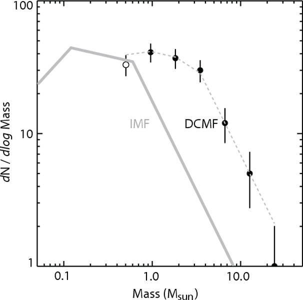 |
Figure 9. Left: extinction map of the Pipe Nebula with the cores circled. Right: mass function of the cores (data points with error bars) compared to stellar IMF (solid line). Reprinted with permission from [46]. |
|
The strong inference from these observations is that, whatever mechanism is responsible for setting the stellar IMF, it acts in the gas phase, before the stars form. In other words, the IMF is simply a translation of the CMF, with only ~ 1/3 of the material in a given core making it onto a star, and the rest being ejected. That ejection fraction is a plausible result of protostellar outflows, as we'll discuss next week. This doesn't by itself represent a theory of the IMF, since it immediately leads to the question of what physical process is responsible for setting the CMF. It does, however, provide an important constraint that what we should be trying to do is to solve three problems: (1) what is responsible for setting the CMF, (2) why is it that cores generally form single stars or star systems regardless of mass, and (3) what sets the efficiency of ~ 1/3.
5.2.3. A Possible Model: Turbulent Fragmentation and Radiation-Suppressed Fragmentation
Although we don't have a complete model that meets the three conditions outlined above, we can sketch out the beginnings of one. This may be entirely wrong, but it's the idea that, right now, I consider the most promising.
The Padoan & Nordlund Model for the CMF The model's basic elements were originally proposed by Padoan & Nordlund [48]. The first element is the idea that supersonic turbulence generates a spectrum of structures with a slope that looks similar to the high end slope of the stellar IMF. Formally, one can show (though we will not in this lecture) that the distribution of fragment masses follows a distribution
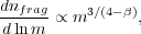 |
(155) |
where  is
a numerical factor related to the exponent q in the
linewidth-size relation by = 2q + 1. (Formally
is the
index of the turbulent power spectrum, so if we have a linewidth-size
relation
is
a numerical factor related to the exponent q in the
linewidth-size relation by = 2q + 1. (Formally
is the
index of the turbulent power spectrum, so if we have a linewidth-size
relation
 v
q,
then one can show that the power spectrum is P(k)
k.) To remind you, for subsonic turbulence q
1/3 and for highly
supersonic turbulence q
1/2, corresponding to
= 5/3 or
= 2,
respectively. At the Mach numbers in molecular clouds
tends to
be a bit less than 2, around 1.9, giving a slope around 1.4. Notice that
this is very similar to the observed high-mass slope
~ 1.3 - 1.4.
v
q,
then one can show that the power spectrum is P(k)
k.) To remind you, for subsonic turbulence q
1/3 and for highly
supersonic turbulence q
1/2, corresponding to
= 5/3 or
= 2,
respectively. At the Mach numbers in molecular clouds
tends to
be a bit less than 2, around 1.9, giving a slope around 1.4. Notice that
this is very similar to the observed high-mass slope
~ 1.3 - 1.4.
By itself this is just a pure powerlaw. However, not all of the structures generated by the turbulence are gravitationally bound and liable to collapse. The very massive ones almost certainly are, because their masses are larger than the Bonnor-Ebert mass for any plausible surface pressure. However, the low mass ones are bound only if they find themselves in regions of high pressure, which lowers the Bonnor-Ebert mass to a value smaller than the mean in the cloud.
To make this more quantitative, recall our result that the distribution
of densities inside a molecular cloud, and thus this distribution of
pressures (since P
in an
isothermal gas), is lognormal. Thus the number of stars formed at a
given mass is given by the number of fragments of that mass produced by
the turbulence multiplied by the probability that each fragment
generated is bound:
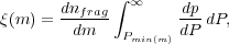 |
(156) |
where Pmin is the minimum pressure required to make an object of mass m unstable, and dP / dp is the (lognormal) distribution of pressures. The effect of this integral is to impose a lognormal turndown on top of the powerlaw produced by turbulence. Simulations seem to show fragments forming in a manner and with a mass distribution that is in good agreement with this model (Figure 10).
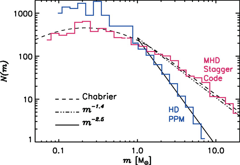 |
Figure 10. The distribution of core masses produced in a simulations of turbulence, using hydrodynamics (blue) and magnetohydrodynamics (red). The overplotted dashed line shows the IMF, using the functional form of [43]. Reprinted with permission from the AAS from [49]. |
The Evolution of Massive Cores
By itself this model is not complete, because it doesn't explain why the
massive cores don't fragment further as they collapse. After all, a 1
M core
may only be about 1 Bonnor-Ebert mass, but a 100
M core
is 100 Bonnor-Ebert masses, so why doesn't it fragment to produce 100
small stars instead of 1 big one? Even for low mass cores there tends to
be too much fragmentation in simulations, resulting in an overproduction
of brown dwarfs compared to what we see.
The answer to that problem was provided in a series of papers by
Krumholz et al.
[51,
52,
53,
54].
Inside a collapsing core a first low mass star will form, and as matter
accretes onto it, the accreting matter releases its gravitational
potential energy as radiation. This is a lot of radiation. In a
massive core the velocity dispersions tend to be supersonic, and the
corresponding accretion rates ~
3 / G
are large, perhaps ~ 10-4 - 10-3
M
yr-1. If one drops mass at this rate onto a protostar of mass
M and radius R, the resulting luminosity is
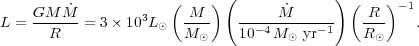 |
(157) |
With a source of this luminosity shining from within it, a massive core
is no longer isothermal. Instead, its temperature rises, raising the
sound speed and suppressing the formation of small stars - recall that,
in an isothermal gas, MBE
cs3
T3/2. Then the problem becomes a dynamical one, in
which there is a competition between secondary fragments trying to
collapse and the radiation from the first object trying to raise their
temperature and pressure to disperse them. One can study this result
using radiation-hydrodynamic simulations, and the result is that, for
sufficiently dense massive cores, the heating tends to win, and massive
cores tend to form binaries, but fragment no further. (This latter point
is good, because essentially all massive stars are observed to be
binaries.)
A final difficulty with massive cores is radiation pressure. A cartoon version of the problem can be understood as follows. Massive stars have very short Kelvin times, so they will reach the main sequence and begin hydrogen burning while they are still accreting. Now consider the force per unit mass exerted by the star's radiation on the gas around it. This is
 |
(158) |
where  is the opacity
per unit mass. We can compare this to the gravitational force per unit
mass
is the opacity
per unit mass. We can compare this to the gravitational force per unit
mass
 |
(159) |
to form the Eddington ratio
 |
(160) |
where the value of
we've plugged in is typical for dusty interstellar gas absorbing near-IR
photons. Thus we expect radiation force to exceed gravitational force
once the star has a light to mass ratio larger than a few thousand in
Solar units. This happens at a mass M ~ 20
M.
So how can bigger stars form, when they should repel rather than attract interstellar matter? This is a classic problem in star formation, and it led to all sorts of exotic theories for how massive stars form, e.g. that they form via stellar collisions in dense clusters. If any of these models are right, then the picture we've just outlined cannot be correct. Fortunately, it turns out that there is a more prosaic answer. Real life is not spherically symmetric, and using radiation to try to hold up infalling gas proves to be an unstable situation. The instability is not all that different from garden variety Rayleigh-Taylor instability, with radiation playing the role of the light fluid (Figure 11).
 |
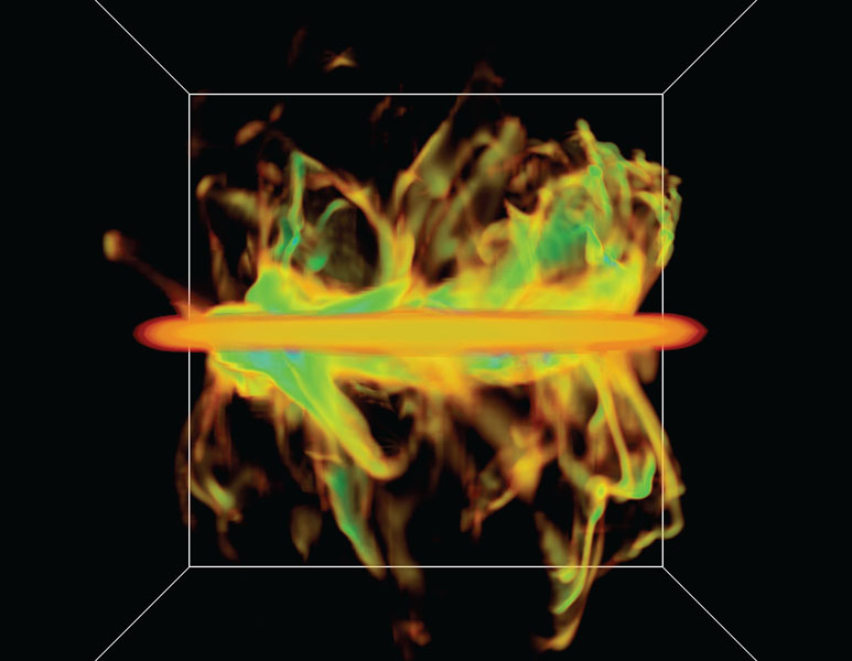 |
Figure 11. A volume rendering of the gas density a simulation of a the formation of a massive binary star system, showing the accretion disk face-on (left) and edge-on (right). Notice the Rayleigh-Taylor fingers that channel gas onto the accretion disk. Reprinted with permission from [50]. |
|
MRK is supported by an Alfred P. Sloan Fellowship; the US National science Foundation through grants AST-0807739 and CAREER-0955300; and NASA through Astrophysics Theory and Fundamental Physics grant NNX09AK31G and a Spitzer Space Telescope Cycle 5 Theoretical Research Program grant.
 0.
IRDCs indicates infrared dark clouds, measured in infrared
absorption. ONC is the Orion Nebula cluster, a single star cluster near
Earth, whose gas mass is estimated from the mass and dynamical state of
the remaining star cluster. HCN represents extragalactic measurements
in the HCN J = 1
0.
IRDCs indicates infrared dark clouds, measured in infrared
absorption. ONC is the Orion Nebula cluster, a single star cluster near
Earth, whose gas mass is estimated from the mass and dynamical state of
the remaining star cluster. HCN represents extragalactic measurements
in the HCN J = 1