


Our modern theory of the structure and evolution of the universe, along with the observational data which support it, is admirably presented in the textbook by Dodelson [4]. Remarkable observational progress has been made in the past two decades which has strengthened our confidence in the correctness of the hot, relativistic, expanding universe model (Big Bang), has measured the universe's present mass-energy contents and kinematics, and lent strong support to the notion of a very early, inflationary phase. Moreover, observations of high redshift supernovae unexpectedly have revealed that the cosmic expansion is accelerating at the present time, implying the existence of a pervasive, dark energy field with negative pressure [5]. This surprising discovery has enlivened observational efforts to accurately measure the cosmological parameters over as large a fraction of the age of the universe as possible, especially over the redshift interval 0 < z < 1.5 which, according to current estimates, spans the deceleration-acceleration transition. These efforts include large surveys of galaxy large scale structure, galaxy clusters, weak lensing, the Lyman alpha forest, and high redshift supernovae, all of which span the relevant redshift range. Except for the supernovae, all other techniques rely on measurements of cosmological structure in order to deduce cosmological parameters.
2.1. Cosmological standard model
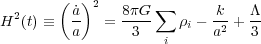
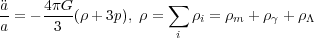
The dynamics of the expanding universe is described by the two Friedmann equations derived from Einstein's theory of general relativity under the assumption of homogeneity and isotropy. The expansion rate at time t is given by
 |
(1) |
where H(t) is the Hubble parameter and a(t)
is the FRW scale factor at time
t. The first term on the RHS is proportional to the sum over
all energy densities in the universe
 i
including baryons, photons, neutrinos, dark
matter and dark energy. We have explicitly pulled the dark energy term out
of the sum and placed it in the third term assuming it is a constant (the
cosmological constant). The second term is the curvature term, where
k = 0, ±1 for zero, positive, negative curvature,
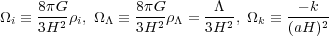
respectively. Equation (1)
can be cast in a form useful for numerical integration if we introduce
i
including baryons, photons, neutrinos, dark
matter and dark energy. We have explicitly pulled the dark energy term out
of the sum and placed it in the third term assuming it is a constant (the
cosmological constant). The second term is the curvature term, where
k = 0, ±1 for zero, positive, negative curvature,
respectively. Equation (1)
can be cast in a form useful for numerical integration if we introduce
 parameters:
 |
(2) |
Dividing equation (1) by H2 we get the sum rule
1 = m +
k +
 ,
which is true at all times,
where m
is the sum over all
i
excluding dark energy. At the present time H(t) =
H0, a = 1, and cosmological density
parameters become
,
which is true at all times,
where m
is the sum over all
i
excluding dark energy. At the present time H(t) =
H0, a = 1, and cosmological density
parameters become
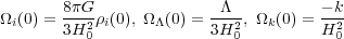 |
(3) |
Equation (1) can then be manipulated into the form
 |
(4) |
Here we have explicitly introduced a density parameter for the background
radiation field
 and used
the fact that matter and radiation
densities scale as a-3 and a-4, respectively,
and we have used the sum rule to eliminate
k.
Equation (4) is equation (1) expressed in terms of the current
values of the density and Hubble
parameters, and makes explicit the scale factor dependence of the various
contributions to the expansion rate. In particular, it is clear that the
expansion rate is dominated first by radiation, then by matter, and finally
by the cosmological constant.
and used
the fact that matter and radiation
densities scale as a-3 and a-4, respectively,
and we have used the sum rule to eliminate
k.
Equation (4) is equation (1) expressed in terms of the current
values of the density and Hubble
parameters, and makes explicit the scale factor dependence of the various
contributions to the expansion rate. In particular, it is clear that the
expansion rate is dominated first by radiation, then by matter, and finally
by the cosmological constant.
Current measurements of the cosmological parameters by different techniques [73] yield the following numbers [(0) notation suppressed]:
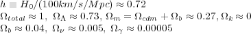 |
This set of parameters is referred to as the concordance model [7], and describes a spatially flat, low matter density, high dark energy density universe in which baryons, neutrinos, and photons make a negligible contribution to the large scale dynamics. Most of the matter in the universe is cold dark matter (CDM) whose dynamics is discussed below. As we will also see below, baryons and photons make an important contribution to shaping of the matter power spectrum despite their small contribution to the present-day energy budget. Understanding the evolution of baryons in nonlinear structure formation is essential to interpret X-ray and SZE observations of galaxy clusters.
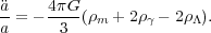
The second Friedmann equation relates the second time derivative of the
scale factor to the cosmic pressure p and energy density
 |
(5) |
p and
are related by an equation of state
pi = wi
i,
with wm = 0, w = 1/3, and
w
= -1. We thus have
 |
(6) |
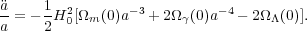
Expressed in terms of the current values for the cosmological parameters we have
 |
(7) |
Evaluating equation 7 using the concordance parameters, we see the
universe is currently accelerating

 0.6H02.
Assuming the dark energy density is a constant, the acceleration began when
0.6H02.
Assuming the dark energy density is a constant, the acceleration began when
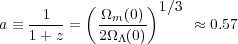 |
(8) |
or z ~ 0.75.
2.2. The Linear power spectrum
Cosmic structure results from the amplification of primordial density
fluctuations by gravitational instability. The power spectrum of matter
density fluctuations has now been measured with considerable accuracy
across roughly four decades in scale. Figure 2
shows the latest results, taken from reference
[8].
Combined in this figure are measurements using cosmic
microwave background (CMB) anisotropies, galaxy large scale structure, weak
lensing of galaxy shapes, and the Lyman alpha forest, in order of
decreasing comoving wavelength. In addition, there is a single data
point for galaxy clusters, whose current space density measures the
amplitude of the power spectrum on 8 h-1 Mpc scales
[9].
Superimposed on the data is the predicted
CDM linear power
spectrum at z = 0 for the concordance model parameters. As one can see, the
fit is quite good. In actuality, the concordance model parameters are
determined by fitting the data. A rather complex statistical machinery
underlies the determination of cosmological parameters, and is discussed in
Dodelson (2003, Ch. 11). The fact that modern CMB and LSS data agree over a
substantial region of overlap gives us confidence in the correctness of the
concordance model. In this section, we define the power spectrum
mathematically, and review the basic physics which determines its shape.
Readers wishing a more in depth treatment are referred to references
[4,
10].
 |
Figure 2. Linear matter power spectrum P(k)
versus wavenumber extrapolated to z = 0, from various measurements of
cosmological structure. The best fit
|
At any epoch t (or a or z) express the matter density in the universe in terms of a mean density and a local fluctuation:
 |
(9) |
where  (
( ) is
the density contrast. Expand
() in
Fourier modes:
) is
the density contrast. Expand
() in
Fourier modes:
 |
(10) |
The autocorrelation function of
() defines
the power spectrum through the relations
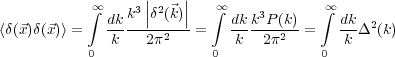 |
(11) |
where we have the definitions
 |
(12) |
The quantity
 2(k)
is called the dimensionless
power spectrum and is an important function in the theory of structure
formation.
2(k)
measures the contribution of perturbations
per unit logarithmic interval at wavenumber k to the variance in
the matter density fluctuations.
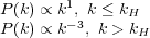
The CDM power
spectrum asymptotes to P(k) ~
k1 for small
k, and P(k) ~ k-3 for large
k, with a peak a k* ~ 2 ×
10-2 h Mpc-1 corresponding to
2(k)
is called the dimensionless
power spectrum and is an important function in the theory of structure
formation.
2(k)
measures the contribution of perturbations
per unit logarithmic interval at wavenumber k to the variance in
the matter density fluctuations.
The CDM power
spectrum asymptotes to P(k) ~
k1 for small
k, and P(k) ~ k-3 for large
k, with a peak a k* ~ 2 ×
10-2 h Mpc-1 corresponding to
 *
~ 350 h-1 Mpc.
2(k)
is thus asymptotically flat at high k, but drops off as
k4 at small k. We therefore see that most of
the variance
in the cosmic density field in the universe at the present epoch is on
scales <
*.
*
~ 350 h-1 Mpc.
2(k)
is thus asymptotically flat at high k, but drops off as
k4 at small k. We therefore see that most of
the variance
in the cosmic density field in the universe at the present epoch is on
scales <
*.
What is the origin of the power spectrum shape? Here we review the basic
ideas.
Within the inflationary paradigm, it is believed that quantum mechanical
(QM) fluctuations in the very early universe were stretched to macroscopic
scales by the large expansion factor the universe underwent during
inflation. Since QM fluctuations are random, the primordial density
perturbations should be well described as a Gaussian random field.
Measurements of the Gaussianity of the CMB anisotropies
[11]
have confirmed this. The primordial power spectrum is parameterized as
a power law Pp
(k)  kn, with n = 1 corresponding to scale-invariant
spectrum proposed by Harrison and Zeldovich on the grounds that any
other value would
imply a preferred mass scale for fluctuations entering the Hubble horizon.
Large angular scale CMB anisotropies measure the primordial power spectrum
directly since they are superhorizon scale. Observations with the WMAP
satellite yield a value very close to n = 1
[73].
kn, with n = 1 corresponding to scale-invariant
spectrum proposed by Harrison and Zeldovich on the grounds that any
other value would
imply a preferred mass scale for fluctuations entering the Hubble horizon.
Large angular scale CMB anisotropies measure the primordial power spectrum
directly since they are superhorizon scale. Observations with the WMAP
satellite yield a value very close to n = 1
[73].
To understand the origin of the spectrum, we need to understand how the
amplitude of a fluctuation of fixed comoving wavelength
grows with
time. Regardless of its wavelength, the fluctuation will pass through
the Hubble horizon as illustrated in Fig. 3.
This is because the Hubble
radius grows linearly with time, while the proper wavelength
a
grows more slowly with time. It is easy to show from Eq. 1 that in
the radiation-dominated era, a ~ t1/2, and in
the matter-dominated era (prior to the onset of cosmic acceleration)
a ~ t2/3. Thus, inevitably,
a fluctuation will transition from superhorizon to subhorizon scale. We are
interested in how the amplitude of the fluctuation evolves during these two
phases. Here we merely state the results of perturbation theory (e.g.,
Dodelson 2003, Ch. 7).
2.3. Growth of fluctuations in the linear regime
To calculate the growth of superhorizon scale fluctuations requires general relativistic perturbation theory, while subhorizon scale perturbations can be analyzed using a Newtonian Jeans analysis. We are interested in scalar density perturbations, because these couple to the stress tensor of the matter-radiation field. Vector perturbations (e.g., fluid turbulence) are not sourced by the stress-tensor, and decay rapidly due to cosmic expansion. Tensor perturbations are gravity waves, and also do not couple to the stress-tensor. A detailed analysis for the scalar perturbations yields the following results. In the radiation dominated era,
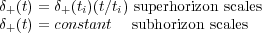 |
This is summarized in Fig. 3, where we consider two fluctuations of different comoving wavelengths, which we will call large and small. The large wavelength perturbation remains superhorizon through matter-radiation equality (MRE), and enters the horizon in the matter dominated era. Its amplitude will grow as t in the radiation dominated era, and as t2/3 in the matter dominated era. It will continue to grow as t2/3 after it becomes subhorizon scale. The small wavelength perturbation becomes subhorizon before MRE. Its amplitude will grow as t while it is superhorizon scale, remain constant while it is subhorizon during the radiation dominated era, and then grow as t2/3 during the matter-dominated era.
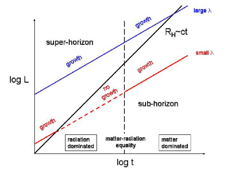 |
Figure 3. The tale of two fluctuations. A fluctuation which is superhorizon scale at matter-radiation equality grows always, while a fluctuation which enters the horizon during the radiation dominated era stops growing in amplitude until the matter dominated era begins. |
Armed with these results, we can understand what is meant by a scale-free
primordial power spectrum (the Harrison-Zeldovich power spectrum.) We are
concerned with perturbation growth in the very early universe during the
radiation dominated era. Superhorizon scale perturbation amplitudes grow as
t, and then cease to grow after they have passed through the
Hubble horizon. We can define a Hubble wave number kH
 2
2 / RH
t-1. Fig. 4a shows the
primordial power spectrum at three instants in time
for k < kH. We see that the fluctuation amplitude at k =
kH(t) depends on primordial power spectrum slope n. The
scale-free spectrum is the value of n such that
2(kH(t)) = constant for
k >
kH. A simple analysis shows that this implies n = 1. Since
2(k)
k3
P(k), we then have
/ RH
t-1. Fig. 4a shows the
primordial power spectrum at three instants in time
for k < kH. We see that the fluctuation amplitude at k =
kH(t) depends on primordial power spectrum slope n. The
scale-free spectrum is the value of n such that
2(kH(t)) = constant for
k >
kH. A simple analysis shows that this implies n = 1. Since
2(k)
k3
P(k), we then have
 |
In actuality, the power spectrum has a smooth maximum, rather than a
peak as shown in Fig. 4c. This smoothing is
caused by the different rates of growth
before and after matter-radiation equality.
The transition from radiation to matter-dominated is not
instantaneous. Rather, the expansion rate of the universe changes smoothly
through equality, as given by Eq. 1, and consequently so do the temporal
growth rates. The position of the peak of the power spectrum is
sensitive to the time when the universe reached matter-radiation
equality, and hence is a probe of
/ m .
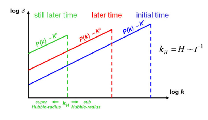 |
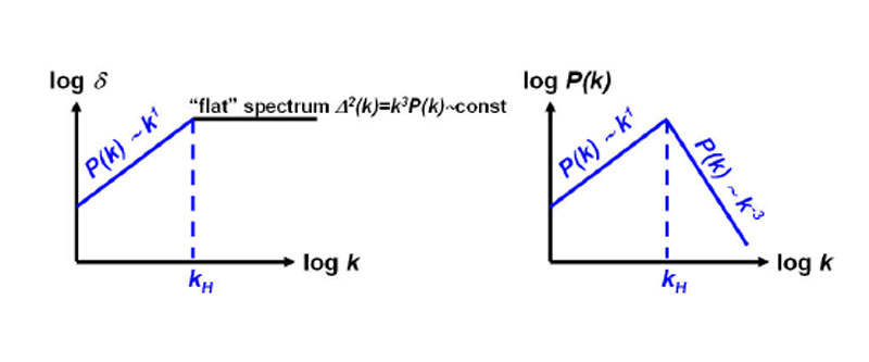 |
Figure 4. a) Evolution of the primordial power spectrum on superhorizon scales during the radiaton dominated era. b) Scale-free spectrum produces a constant contribution to the density variance per logarithmic wavenumber interval entering the Hubble horizon (no preferred scale) c) resulting matter power spectrum, super- and sub-horizon. Figures courtesy Rocky Kolb. |
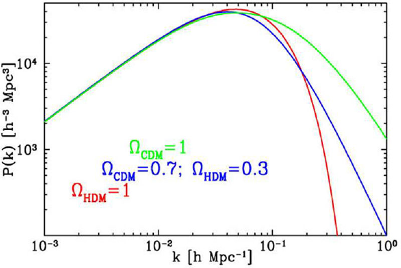
Once a fluctuation becomes sub-horizon, dissipative processes modify the shape of the power spectrum in a scale-dependent way. Collisionless matter will freely stream out of overdense regions and smooth out the inhomogeneities. The faster the particle, the larger its free streaming length. Particles which are relativistic at MRE, such as light neutrinos, are called hot dark matter (HDM). They have a large free-streaming length, and consequently damp the power spectrum over a large range of k. Weakly Interacting Massive Particles (WIMPs) which are nonrelativistic at MRE, are called cold dark matter (CDM), and modify the power spectrum very little (Fig. 5). Baryons are tightly coupled to the radiation field by electron scattering prior to recombination. During rcombination, the photon mean-free path becomes large. As photons stream out of dense regions, they drag baryons along, erasing density fluctuations on small scales. This process is called Silk damping, and results in damped oscillations of the baryon-photon fluid once they become subhorizon scale. The magnitude of this effect is sensitive to the ratio of baryons to collisionless matter, as shown in Fig. 5.
 |
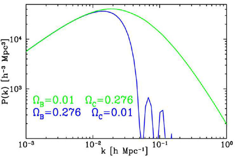 |
Figure 5. Effect of dissipative processes on the evolved power spectrum. Left: Effect of collisionless damping (free streaming) in the dark matter. Right: Effect of collisional damping (Silk damping) in the matter-radiation fluid. Figures courtesy Rocky Kolb. |
|