3. ANALYTIC MODELS FOR NONLINEAR GROWTH, VIRIAL SCALING RELATIONS, AND HALO STATISTICS

Here we introduce a few concepts and analytic results from the theory of structure formation which underly the use of galaxy clusters as cosmological probes. These provide us with the vocabulary which pervades the literature on analytic and numerical models of galaxy cluster evolution. Material in this section has been derived from three primary sources: Padmanabhan (1993) [12] for the spherical top-hat model for nonlinear collapse, Dodelson (2003) [4] for Press-Schechter theory, and Bryan & Norman (1998) [13] for virial scaling relations.

3.1. Nonlinearity defined

In the linear regime, both super- and sub-horizon scale perturbations grow as t^2/3 in the matter-dominated era. This means that after recombination, the linear power spectrum retains its shape while its amplitude grows as t^4/3 before the onset of cosmic acceleration (Fig. 6a). When ²(k) for a given k approaches unity linear theory no longer applies, and some other method must be used to determine the fluctuation's growth. In general, numerical simulations are required to model the nonlinear phase of growth because in the nonlinear regime, the modes do not grow independently. Mode-mode coupling modifies both the shape and amplitude of the power spectrum over the range of wavenumbers that have gone nonlinear.

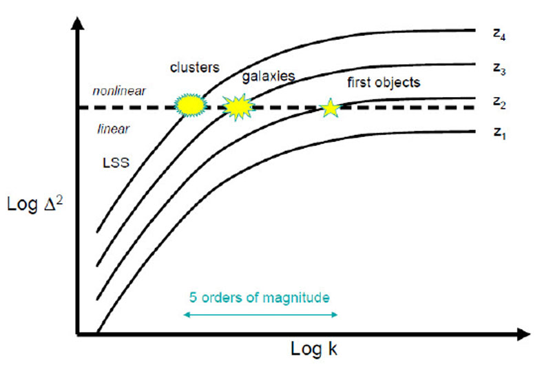Figure 6. Two ways of looking at the growth of post-recombination matter fluctuations in the linear regime. Left: 3D matter power spectrum increases uniformly proportional to the linear growth factor D(z). Measurements are from SDSS galaxy large scale structure data. Right: the evolution of the dimensionless power spectrum 2(k). Nonlinearity is defined where 2(knl) = 1. All scales with k knl have collapsed into bound objects, and do so in a "bottom-up" fashion.

At any given time, there is a critical wavenumber which we shall call the nonlinear wavenumber k_nl which determines which portion of the spectrum has evolved into the nonlinear regime. Modes with k < k_nl are said to be linear, while those for which k > k_nl are nonlinear (Fig. 6b). Conventionally, one defines the nonlinear wavenumber such that (k_nl, z) = 1. From this one can derive a nonlinear mass scale M_nl(z) = (4 / 3) (z) (2 / k_nl)³. A more useful and rigorous definition of the nonlinear mass scale comes from evaluating the amplitude of mass fluctuations within spheres or radius R at epoch z. The enclosed mass is M = (4 / 3) (z) R³. The mean square mass fluctuations (variance) is

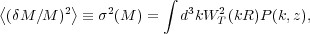(13)

where W is the Fourier transform of the top-hat window function

(14)

If we approximate P(k) locally with a power-law P(k,z) = D²(z) k^m, where D is the linear growth factor, then ²(M) D² R^{-(3 + m)} D² M^{-(3 + m)/3}. From this we see that the RMS fluctuations are a decreasing function of M. At very small mass scales, m -3, and the fluctuations asymptote to a constant value. We now define the nonlinear mass scale by setting (M_nl) = 1. We get that ([17])

(15)

For m > -3, the smallest mass scales become nonlinear first. This is the origin of hierarchical ("bottom-up") structure formation (Fig. 6b).

3.2. Spherical Top-Hat Model

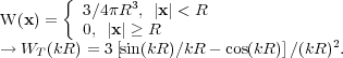
We now ask what happens when a spherical volume of mass M and radius R exceeds the nonlinear mass scale. The simplest analytic model of the nonlinear evolution of a discrete perturbation is called the spherical top-hat model. In it, one imagines as spherical perturbation of radius R and some constant overdensity = 3M / 4 R³ in an Einstein-de Sitter (EdS) universe. By Birkhoff's theorem the equation of motion for R is

(16)

whereas the background universe expands according to Eq. 6

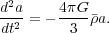(17)

Comparing these two equations, we see that the perturbation evolves like a universe of a different mean density, but with the same initial expansion rate. Integrating Eq. 16 once with respect to time gives us the first integral of motion:

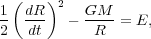(18)

where E is the total energy of the perturbation. If E < 0, the perturbation is bound, and obeys

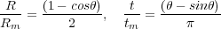(19)

where R_m and t_m are the radius and time of "turnaround". At turnaround (as ), the fluctuation reaches its maximum proper radius (see Fig. 7). As t 2t_m, R 0, and we say the fluctuation has collapsed.

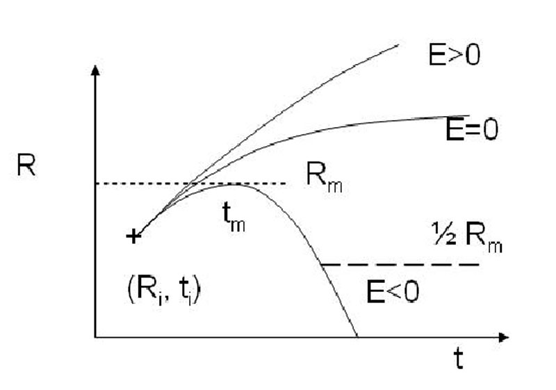Figure 7. Evolution of a top-hat perturbation in an EdS universe. Depending on the E, the first integral of motion, the fluctuation collapses (E < 0), continues to expand (E > 0), or asymptotically reaches it maximum radius (E = 0). Virialization occurs when the fluctuation has collapsed to half its turnaround radius.

3.3. Virial Scaling Relations

The spherical top-hat model can be scaled to perturbations of arbitrary mass. Using virial equilibrium arguments, we can predict various physical properties of the virialized object. The ones that interest us most are those that relate to the observable properties of gas in galaxy clusters, such as temperature, X-ray luminosity, and SZ intensity change. Kaiser [14] first derived virial scaling relations for clusters in an EdS universe. Here we generalize the derivation to non-EdS models of interest. In order to compute these scaling laws, we must assume some model for the distribution of matter as a function of radius within the virialized object. A top-hat distribution with a density = _c (z) is not useful because it is not in mechanical equilibrium. More appropriate is the isothermal, self-gravitating, equilibrium sphere for the collisionless matter, whose density profile is related to the one-dimensional velocity dispersion [15]

(20)

If we define the virial radius r_vir to be the radius of a spherical volume within which the mean density is _c times the critical density at that redshift (M = 4 r_vir³ _{crit c} / 3), then there is a relation between the virial mass M and :

(21)

Here we have introduced a normalization factor f which will be used to match the normailization from simulations. The redshift dependent Hubble parameter can be written as H(z) = 100hE(z) km s^-1 with the function E²(z) = _m (1 + z)³ + _k (1 + z)² + , where the 's have been previously defined.

The value of _c is taken from the spherical top-hat model, and is 18² for the critical EdS model, but has a dependence on cosmology through the parameter (z) = _m (1 + z)³ / E²(z). Bryan and Norman (1998) provided fitting formulae for _c for the critical for both open universe models and flat, lambda-dominated models

(22)

where x = (z) - 1.

If the distribution of the baryonic gas is also isothermal, we can define a ratio of the "temperature" of the collisionless material (T = µ m_p ² / k) to the gas temperature:

(23)

Given equations (22) and (23), the relation between temperature and mass is then

(24)

where in the last expression we have added the normalization factor f_T and set = 1.

The scaling behavior for the object's X-ray luminosity is easily computed by assuming bolometric bremsstrahlung emission and ignoring the temperature dependence of the Gaunt factor: L_bol ² T^1/2 dV M_b T^1/2. where M_b is the baryonic mass of the cluster. This is infinite for an isothermal density distribution, since is singular. Observationally and computationally, it is found that the baryon distribution rolls over to a constant density core at small radius. A procedure is described in Bryan and Norman (1998) which yields a finite luminosity:

(25)

Eliminating M in favor of T in Eq. 25 we get

(26)

The scaling of the SZ "luminosity" is likewise easily computed. If we define L_SZ as the integrated SZ intensity change: L_SZ = dA n_{e T}( kT / (m_ec²))dl M_b T, then

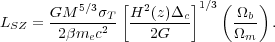(27)

We note that cosmology enters these relations only with the combination of parameters h² _c E², which comes from the relation between the cluster's mass and the mean density of the universe at redshift z. The redshift variation comes mostly from E(z), which is equal to (1 + z)^3/2 for an EdS universe.

3.4. Statistics of hierarchical clustering: Press-Schechter theory

Now that we have a simple model for the nonlinear evolution of a spherical density fluctuation and its observable properties as a function of its virial mass, we would like to estimate the number of virialized objects of mass M as a function of redshift given the matter power spectrum. This is the key to using surveys of galaxy clusters as cosmological probes. While large scale numerical simulations can and have been used for this purpose (see below), we review a powerful analytic approach by Press and Schechter [16] which turns out to be remarkably close to the numerical results. The basic idea is to imagine smoothing the cosmological density field at any epoch z on a scale R such that the mass scale of virialized objects of interest satisfies M = (4 / 3) (z)R³. Because the density field (both smoothed and unsmoothed) is a Gaussian random field, the probability that the mean overdensity in spheres of radius R exceeds a critical overdensity _c is

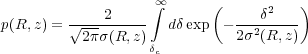(28)

where (R, z) is the RMS density variation in spheres of radius R as discussed above. Press and Schechter suggested that this probability be identified with the fraction of particles which are part of a nonlinear lump with mass exceeding M if we take _c = 1.686, the linear overdensity at virialization. This assumption has been tested against numerical simulations and found to be quite good [9] (however, see below). The fraction of the volume collapsed into objects with mass between M and M + dM is given by (dp / dM)dM. Multiply this by the average number density of such objects _m /M to get the number density of collapsed objects between M and M + dM:

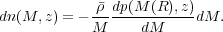(29)

The minus sign appears here because p is a decreasing function of M. Carrying out the derivative using the fact that dM / dR = 3M / R, we get

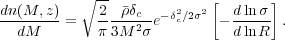(30)

The term is square brackets is related to the logarithmic slope of the power spectrum, which on the mass scale of galaxy clusters is close to unity. Eq. 30 is called the halo mass function, and it has the form of a power law multiplied by an exponential. To make this more explicit, approximate the power spectrum on scales of interest as a power law as we have done above. Substituting the scaling relations for in Eq. 30 one gets the result [17]

(31)

Here, M_nl(z) is the nonlinear mass scale. To be more consistent with the spherical top-hat model, it satisfies the relation (M_nl, z) = _c ; i.e., those fluctuations in the smoothed density field that have reached the linear overdensity for which the spherical top-hat model predicts virialization.

3.5. Validating the Halo Mass Function using N-body Simulations

Below we discuss how one goes about numerically simulating the nonlinear evolution of the density fluctuations described by the CDM power spectrum. Here we simply mention two works which made detailed comparisons of the PS formula with halo populations found in dark matter N-body simulations. The first is by Jenkins et al. (2001) [74] who analyzed the results of the "Hubble Volume" simulation - a simulation of dark matter clustering carried out in a cubic volume 3 Gpc/h on a side with 1024³ dark matter particles (Fig. 8). This yields a dark matter particle mass of 2.2 × 10¹² M, implying that a galaxy cluster halo would typically contain 100-1000 particles. The relatively poor mass resolution is offset by the very large volume, which permits exploring the cluster mass function across a broad range of masses including the very high mass end. Fig. 8 shows a slice through the simulation volume on which the dark matter density field is plotted. Jenkins et al. (2001) identified dark matter halos using the friends-of-friends algorithm [52] and found that while the PS formula gives a good approximation to the numerical data, it underpredicts the number of rare, massive objects, and overpredicts the number of "typical" objects as shown in the right panel of Fig. 8.

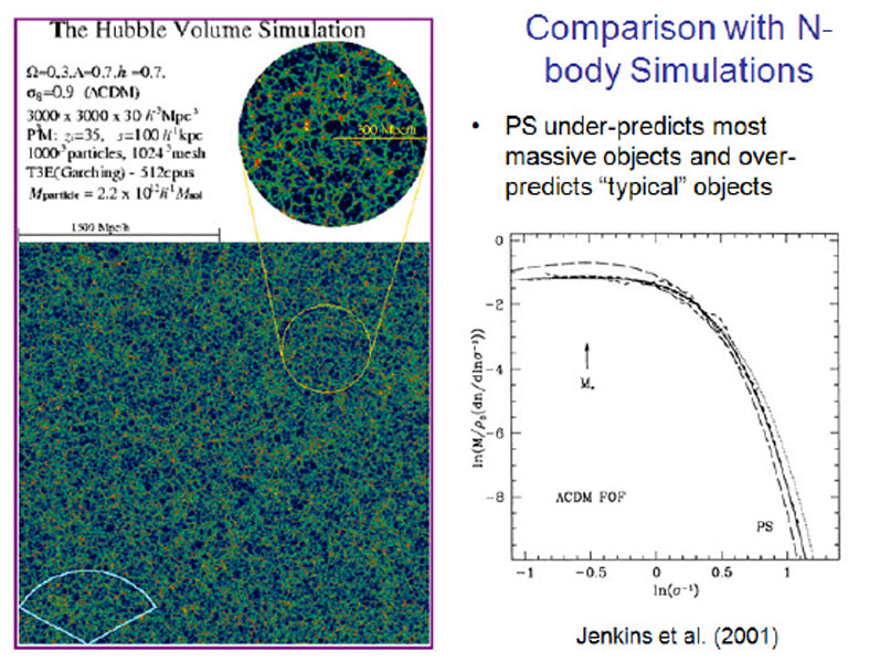Figure 8. The Hubble Volume Simulation [76]. Left: slice through the dark matter density field. Yellow/orange peaks correspond to galaxy clusters. Right: Halo multiplicity function, as measured from the simulation (solid lines), with Press-Schechter prediction superposed (dashed line). From [74].

Warren et al. (2006) [75] were interested in testing the validity of the PS formula over a wider range of mass scales than can be obtained from a single simulation. They simulated 16 boxes of different physical size but the same number of DM particles (1024³) nested in such a way that together they define a composite halo mass function covering 5 orders of magnitude in mass scale. They derived a fitting formula for the composite halo mass function for the WMAP3 concordance cosmological parameters by assuming a parameterized form for the halo multiplicity function of:

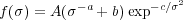(32)

where the multiplicity function f() is related to the mass function n(M) via

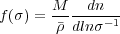(33)

where A, a, b and c come from the fitting procedure, and are documented in [75].

To illustrate one application of this formula, Fig. 9 shows the cluster halo mass function computed using the Warren et al. (2006) fit for three different redshifts for the cosmological parameters adopted in the simulation shown in Fig. 1. Overplotted on the semi-analytic predictions are the halo mass functions obtained from the simulation itself. The departure of the simulation from the predictions at the low mass end are due to finite resolution effects discussed in Sec. 4 below.

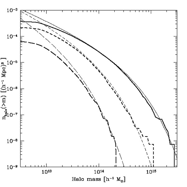Figure 9. Cumulative number of galaxy clusters exceeding mass m for three redshifts. Solid lines: z = 0.1, short-dashed lines z = 1, long-dashed lines z = 2. The thick lines are from the simulation shown in Fig. 1, while the thin lines are predictions using the Warren [75] fitting function. Note the rapid redshift evolution of the number of massive clusters. The departure of the simulation from the predictions at the low mass end are due to finite resolution effects. From [77].

3.6. Application to galaxy clusters

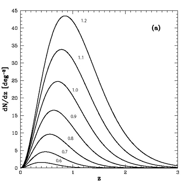
The aerial density of galaxy clusters can be calculated by multiplying the redshift-dependent halo mass function using the Warren fitting formula with the redshift-dependent differential volume element for one square degree on the sky. Fig. 10a shows the result varying the amplitude of the matter power spectrum ₈ holding all other cosmological parameters fixed, while Fig. 10b shows the result varying the matter density _m holding all other cosmological parameters fixed. In general we see a rapid rise in the number of clusters with increasing redshift due to the increasing volume element. However, the space density of clusters declines rapidly with redshift (see Fig. 9), and thus the aerial density peaks at z 1 and then declines rapidly toward higher redshift.

Figure 10. Predicted aerial density of galaxy clusters for the WMAP3 concordance cosmological model. Left: varying the amplitude of the matter power spectrum 8 holding all other parameters fixed; Right: varying the matter density m holding all other parameters fixed. From [77].

From these curves and the virial scaling relations given above it is easy to predict the expected number of clusters of a given X-ray temperature, X-ray luminosity, or SZ luminosity as a function of redshift [18, 13], bearing in mind that real clusters may not perfectly obey the virial scaling relations. In fact they don't as discussed in my 2004 Varenna lectures [69] and by Borgani in these proceedings.