8.2. STAR FORMATION

Here I describe the various probes of star formation in galaxies and their correlation with the molecular gas contents. I devote considerable effort to developing an interpretive framework for the FIR emission from optically thick dust clouds.

8.2.1. Probes of star formation

There are a number of observational tracers which have been developed to measure the star formation rates (SFRs) in galaxies (see Calzetti, this volume). The Hi recombination lines in the visible and near-IR (e.g., H and P) have the fluxes proportional to the Hii region emission measures, hence the OB star formation rate over the last 10⁷ yr. The restframe (far-)UV continuum ([F]UV), at < 2000 Å, arising from hot, early-type stars has been used to infer the SFRs for large samples of galaxies. Both the emission lines and the UV continuum can be severely attenuated by dust extinction in star-forming regions. Even for the galaxies with detected UV continuum, the extinction corrections are often factors of 5-10! For the dust-obscured star formation, the FIR luminosity (_rest = 8-1000 µm) provides a much more reliable measure of the SFR. These FIR SFRs can now be obtained for large samples of galaxies using observations from the Spitzer and Herschel space telescopes, albeit with relatively low angular resolution and sensitivity to SFR (compared to the UV). A summary of all these techniques, including relevant SFR equations, appears in the recent paper by Murphy et al. (2011) so I will not detail all of them here - instead I will focus on developing a physical understanding of the IR emission.

8.2.2. Infrared emission

The FIR emission from both star-forming and active galactic nucleus (AGN) sources arises from dust surrounding these sources which has been radiatively heated by absorption of the outflowing photons. Here I develop the logical steps for interpreting the IR emission since I have not seen this done systematically elsewhere.

The dust temperatures are determined by radiative equilibrium at distance R from a central source of luminosity L, with

(9)

where a_d and T_d are the dust grain radius and temperature, and < > and <> are the dust emission and absorption efficiencies (shown in Fig. 8.7, left panel), weighted, respectively, by the Planck spectrum at the local dust temperature and that of the luminosity source heating the dust. If the emission efficiency varies as 1/, i.e., T_d, then

(10)

(Goldreich & Kwan 1974). More generally,

(11)

where <(T)> and <(T)> are shown in the right panel of Fig. 8.7. Due to the flatness of the broadband absorption coefficient from 2 to 50 µm, the grain absorption and emission efficiencies integrated over black-body spectra are decreasing only modestly from T_BB = 1000-100 K (Fig. 8.7, right).

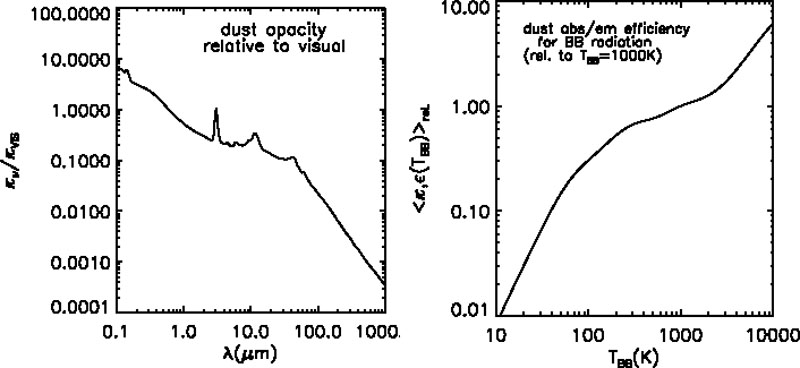Figure 8.7. Left panel: the dust absorption opacity as a function of wavelength (Isella et al. 2010) for standard interstellar grain composition (12% silicates, 27% organics, and 61% water ice; Pollack et al. 1994), and size distribution n(a) a-3.5 from 0.01 to 1 µm radius. The absorption coefficient is normalised relative to that at visual wavelength (6060 Å, V = 2.3 × 104 gr-1) - for a standard gas-to-dust abundance (~ 100 in mass) with NH+2H2 = 2 × 1021 cm-2 per mag of visual extinction (AV). An important feature of the extinction curve is the relatively flat broadband absorption coefficient over the range = 2-50 µm. In the right panel, I show the Planck integrated absorption/emission coefficient as a function of blackbody temperature. Due to the `flat' absorption coefficient in the near- and mid-IR (NIR/MIR), the Planck-integrated absorption and emission efficiency is quite independent of temperature from 1000 K down to 100 K. The dust opacity curve was calculated by Andrea Isella and is available from him or myself.

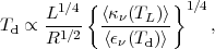
Figure 8.8 shows the computed dust temperatures for the optically thin and optically thick cases, evaluated from Equation 8.11. In the optically-thick regime, the fall-off in dust temperature is r^-1/2 - an extremely simple form due to the fact that the photons heating the grains and those emitted by the grains have similar wavelength distributions. One will therefore have <> ~ <> in the very optically-thick dust clouds.

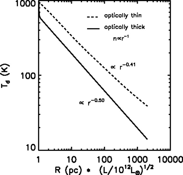Figure 8.8. The temperature of dust heated by a central luminosity source is shown as a function of radius for optically thin dust (with all the heating provided by a ~ 104 K blackbody) and for very optically thick dust (where after the innermost radius, the heating is due to dust at the same radius and temperature). This resembles closely the very optically-thick case since the temperature gradients are generally quite shallow. It is important to appreciate that the radial physical scalelengths will simply stretch homologously with changing source luminosity. 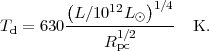Thus the same curves can be used for sources with very much higher or lower luminosity. For optically-thick FIR dust emission the dust temperature varies as Td r-1/2. In real emission sources, the dust is optically thin right at the inner boundary, optically thick at intermediate radii and then thin at the outer radii so the temperature profiles must be pieced together at the appropriate radii. (These equilibrium dust temperatures were calculated using the grain absorption coefficients shown in Fig. 8.7 and the inner boundary is taken to be where the grain temperature is ~ 1000 K, i.e., somewhat below the expected dust sublimation temperatures.)

The radial scale in Fig. 8.8 is for a central source luminosity of 10¹² L, appropriate to ULIRGs and submm galaxies (SMGs), but the radial distances can be scaled as L^1/2 for other luminosities (see Equation 8.11). Thus, these temperature profiles can be equally well applied to a dust cloud surrounding a luminous protostellar cluster of luminosity 10³-10⁶ L. The temperature profiles in Fig. 8.8 start at ~1000 K which is a little below the dust sublimation temperatures ( 1500 K). Inside this radius, the dust will not survive. For a less luminous source, this inner radius will scale inwards; but the physical scales will all change by the same L^1/2 and the modelling remains homologous.

8.2.3. Dust optical depth: < 1 or > 1 ?

It is quite trivial to observationally distinguish the optically thick and thin sources since the latter will have a power-law flux distribution on the short-wavelength side of the peak whereas the former will appear more exponential (see Scoville & Kwan 1976). (If the dust distribution is clumpy, photons can emerge from the inner regions with hot dust - thus, in optically-thick dust clouds, a non-exponential spectral energy distribution [SED] at short wavelengths might also occur; see Fig. 8.17.)

Virtually all IR sources associated with active star-forming regions (Galactic GMCs and starburst nuclei) are optically thick into the MIR (based on their sharp short wavelength fall-off). Since the dust opacity is fairly flat across the wavelength range (2-50 µm), one then expects that the source will become optically thin only at > 50 µm, as long as it is optically thick at 3-10 µm. Thus, it is most appropriate to employ the optically thick dust temperature distribution shown as a solid line in Fig. 8.8 and fit numerically by

(12)

One can invert Equation 8.12 to find the characteristic size of the emitting region:

(13)

if the total IR luminosity and dust temperature are known. The latter might be derived by fitting the MIR SED, or more crudely, from the wavelength of the peak. If the dust is opaque, then the standard Planck expression yields T_d = 100 × (51 µm / _peak) K but if the dust is optically thin, then the peak wavelength is reduced by a factor ~ (3 / (3 + )) where is the power-law index for the opacity, , near the IR peak.

In practice, the opacity can never be much greater than unity at the peak. This is due to the simple fact that the luminosity cannot escape from the inner regions which have high opacity to the cloud surface. And once the outward luminosity flux has shifted to wavelengths where the opacity becomes less than unity, it escapes. This can be seen analytically using the fact that the emergent emission for a given grain is proportional to B e^(-). At > 70 µm, ^~1.6. If = ( / ₀)^1.6 (i.e., unity at = ₀), then the emission of the grain will peak at _m (3 + 1.6)₀ / (1.6 + h₀ / kT_d), where = (_m / ₀)^1.6. Thus, for example, with T_d = 100 K, the blackbody peak at 51 µm is shifted to 78 and 395 µm for ₀ = 102 and 787 µm, respectively. At the peaks the optical depths are _peak = 1.5 and 3.0 in the two cases. This illustration was for an isothermal dust distribution with simplistically representing the foreground optical depth. This also provides a strong note of caution - if one is deriving the dust temperature from the wavelength of peak emission, the peak will usually be shifted to a longer wavelength where the dust starts to become transparent.

8.2.4. Dust temperature of the emergent luminosity

So how can the characteristic dust temperatures be derived? Probably the best approach, if the dust is believed to be optically thick on the short wavelength side of the peak (based on an `exponential' rise), is to simply assume that ~ 1 at the peak and estimate the temperature of the dust emitting the bulk of the emergent luminosity from T_d 100 × (80 µm / _peak) K. To improve on this ad hoc correction requires an assumption of the dust density distribution with radius and modelling the emergent SED (as is done below in Section 8.2.9).

For an optically-thick source, the emergent radiation at each wavelength will be from a depth where 1. Since the dust opacity falls off at longer wavelengths and the temperature is falling at larger radii, this implies, somewhat counter-intuitively, that at wavelengths short of the peak wavelength, one will sample dust at increasingly larger radii, i.e., lower and lower temperatures!

8.2.5. Star formation rate from L_IR

Derivation of SFRs from the IR luminosities is fairly straightforward and robust. This was first done by Scoville & Young (1983) using the fact that the bulk of the luminosity from a stellar population at early times is generated largely by the OBA stars. For those stars an approximately fixed percentage (13%) of their initial mass gets processed through the CNO cycle and one knows the energy produced per CNO process. This derivation is analogous to the `fuel consumption theorem' of Renzini & Buzzoni (1986).

A more precise, modern approach is to run starburst models (e.g., Starburst99; Leitherer et al. 1999) and integrate up the luminosity as a function of time. One must assume a stellar initial mass function (IMF), and its mass range, and decide which photons will be absorbed by dust and for how long the dust absorption persists. In Fig. 8.9 I show results obtained using Starburst99 with a Kroupa IMF (0.1 to 100 M, Kroupa 2001) as a function of the duration of the dust absorption. The latter quantity is probably ~ 10⁷ yr for Galactic star-forming regions but could be closer to 10⁸ yr for merging starburst galaxies where the dust is more widely distributed. For this calculation, I assume all stellar and nebular photons longward of the Lyman limit (912 Å) are absorbed by the surrounding dust. From Fig. 8.9, one could reasonably compute a SFR given by

(14)

with the lower value being appropriate to the ULIRGs which have longer duration for the dust shrouding. The standard relation given by Murphy et al. (2011) corresponds to 1.5 × 10^-10 M yr^-1 (L_IR / L). The simpler derivation outlined above (based on the CNO cycle energy production) is quite similar to Equation 8.14 after one corrects for the mass going into non-OBA stars for a Kroupa IMF.

Figure 8.9. The conversion of observed IR luminosities into estimates of the SFR depends on the duration time of the dust absorption. Here I have used Starburst99 models with a Kroupa IMF and assumed that all stellar and nebular photons longward of the Lyman limit are absorbed for the dust duration time (in Myr) and then none are absorbed after that. For normal star-forming regions this timescale is ~ 10 Myr and for ULIRGs 50-100 Myr. If the dust envelope lasts less than 10 Myr and or is only partially covering, then the conversion factor is significantly higher - both are certainly true for an exposed Hii region like the Orion nebula.

8.2.6. Dust and ISM mass estimates

On the long-wavelength Rayleigh-Jeans (R-J) tail of the FIR emission, the dust will be optically thin and the observed continuum fluxes provide an excellent means of determining the overall mass of dust. If the dust-to-gas abundance is normal, this dust mass can then be scaled to estimate the overall mass of ISM within a star-forming region or a distant galaxy.

On the optically-thin R-J tail of the IR emission, the observed flux density is given by

(15)

or in terms of the dust opacity per unit gas mass, (ISM) = × M_dust / M_ISM,

(16)

where d_l is the source luminosity distance. In normal star-forming galaxies, the majority of the dust is at ~ 20-25 K, and even in the most vigorous starbursts like Arp 220 the FIR/submm emission is dominated by dust at temperatures 45 K. Thus the expected variations in T_dust have less than a factor two effect on the observed flux.

The dust opacity per unit mass of total ISM gas, (ISM) in Equation 8.16, can be calibrated from the extensive submm observations of nearby galaxies. Seventeen of the nearby SINGS survey (Spitzer Infrared Nearby Galaxies Survey; Kennicutt et al. 2003) galaxies have good total submm flux measurements obtained with the SCUBA instrument, mounted at the James Clerk Maxwell Telescope, at 850 µm (see Draine et al. 2007), as well as good measurements of the total molecular (H₂) and atomic (Hi) gas masses.

In Fig. 8.10, the derived dust-to-gas (H₂ + Hi) mass ratios from Draine et al. (2007) are shown for the galaxies having SCUBA 850 µm measurements, for a range of spiral type (Sa to Sd) and as a function of mean metallicity. (Equivalent data for low-redshift elliptical galaxies are not available from Draine et al. 2007 due to lack of gas mass measurements in the early type galaxies.)

Figure 8.10. Left panel shows the dust-to-gas mass ratios derived by Draine et al. (2007) for galaxies from the SINGS nearby galaxy survey, selecting only those galaxies with both SCUBA 850 µm fluxes and complete maps of the H2 and Hi gas; right panel shows the mass-metallicity relation for low-z galaxies (grey points) and binned values for z ~ 2 galaxies (red dots) from Erb et al. (2006). Over a range of 0.5 dex in metallicity below that of the Milky Way there is little variation in the dust-to-gas ratios. Since the galaxies selected here are massive, their metallicities even at z = 2 are expected to be within this range based on emission line ratios. Lower-metallicity irregular galaxies probably do show a decrease in the dust abundance (see Draine et al. 2007).

Figure 8.10 shows that over a range of ~ 0.5 dex in metallicity, there is little empirical evidence of variation in the dust-to-gas mass ratios and hence the submm flux. If one includes even lower-metallicity galaxies that do not have SCUBA 850 µm fluxes (hence the submm fluxes must be extrapolated from an overall SED fit using shorter-wavelength observations), there is evidence for a metallicity dependence in the dust-to-gas ratio. Lastly, it should be emphasised that although some variations in the ratio of submm flux to ISM mass may be expected, ISM mass estimates at ~ 30% accuracy (see Fig. 8.10) are still likely to be at least as accurate as those from CO line measures and much quicker, enabling large samples to be analysed.

In view of the large uncertainty in the submm absorption coefficient and its scaling with frequency, we adopt an empirical approach based on submm observations of local galaxies where Hi and H₂ masses have been estimated. For the local galaxies on which to base this empirical approach, it is vital that both the submm fluxes and ISM masses are global values. In addition as a check on the reliability of the submm measurements we require two long wavelength flux measurements so one can check if there is reasonable consistency with expected values of the spectral index .

For the spectral index of the R-J tail (S varying as ), the observed flux ratios of submm galaxies can vary between 3 and 4. For most dust models the spectral index of the opacity is typically 1.5 to 2, implying = 3.5 to 4. Empirical fits to the observed long wavelength SEDs give = 3.5 to 4 (Dunne & Eales 2001; Clements et al. 2010) for local galaxies. For high-z submm galaxies, the spectral index can be between 3.2 and 3.8, but in most cases the shorter-wavelength point is getting close the IR peak in the restframe and therefore not strictly on the R-J tail. In the following, we adopt = 3.8.

Table 8.1 lists local spiral or star-forming galaxies for which both 450 and 850 µm measurements exist with good signal-to-noise and for which global fluxes were estimated.

Table 8.1. Low-z galaxies with submm & ISM data

Galaxy	Distance	S(450 µ)	S(850 µ)	logMHI	logMH2
	(Mpc)	(Jy)	(Jy)	(M)	(M)
NGC 4631	9.0	30.7	5.73	9.2	9.5
NGC 7331	15.7	18.5	2.98	9.4	9.7
NGC 7552	22.3	20.6	2.11	9.7	10.0
NGC 598	76.0	2.3	0.26	9.8	10.1
NGC 1614	62.0	1.0	0.14	9.7	10.0
NGC 1667	59.0	1.2	0.16	9.3	9.6
Arp 148	143.0	0.6	0.09	9.9	10.2
1 ZW 107	170.0	0.4	0.06	10.0	10.3
Arp 220	79.0	6.3	0.83	10.0	10.3
12112+0305	293.0	0.5	0.05	10.3	10.6
Mrk 231	174.0	0.5	0.10	9.8	10.1
Mrk 273	153.0	0.7	0.08	9.9	10.2

The 850 µm fluxes were then converted to specific luminosity L₍₈₅₀₎, using

(17)

Figure 8.11. The ratio of L at 850 µm to MISM is shown for a sample of low-z spiral and starburst galaxies from Dale et al. (2005) and Clements et al. (2010). The average and median values for the sample are shown by horizontal lines.

Figure 8.11 shows the ratio L₈₅₀ / M_ISM as a function of L₈₅₀ where M_ISM = M_HI + M_H2. Based on this plot, we then adopt as a working value

(18)

Define this mean value as

(19)

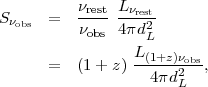
For high-redshift observations,

(20)

with

(21)

Therefore,

(22)

with

(23)

Then,

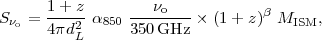(24)

where the 350 GHz is the frequency corresponding to 850 µm.

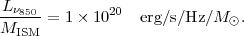
Normalising to M_ISM = 2 × 10¹⁰ M with = 3.8,

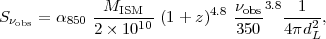(25)

(26)

at z = 0.3, 1, 2 and 3, d_L(Gpc) = 1.5, 6.6, 15.5 and 25.4 Gpc.

Figure 8.12 shows the new predicted fluxes as a function of redshift for both Band 6 (240 GHz) and Band 7 (347 GHz).

Figure 8.12. The expected ALMA Band 6 (240 GHz) and Band 7 (345 GHz) flux densities are shown for MISM = 2 × 1010 M.

For reference, looking at the ALMA exposure time calculator, with 7.5 GHz bandwidth in each polarisation and 10.2 min of integration at Cycle 1 yields 1 = 0.075 mJy at 345 GHz, 1 = 0.042 mJy at 240 GHz and 0.029 mJy at 100 GHz. The expected fluxes on Fig. 8.12 for z = 2 are ~ 1.7 and 0.3 mJy respectively for 2 × 10¹⁰ M. Thus Band 7 is optimal since the expected flux ratio is ~ 5:1. Band 3 (100 GHz) is not plotted in the figure since its expected flux density is 28 times below that of Band 6.

To compare with the ability to detect CO, we might use the source BX 691 from Tacconi et al. (2010) which has a M_* = 7.6 × 10¹⁰ M and M_H2 = 3.5 × 10¹⁰ M at z = 2.19 and CO(3-2) = 0.15 Jy km s^-1. For a width of 300 km s^-1, this has an average line flux of 0.5 mJy. If the mass is scaled to 2 × 10¹⁰ M, then the average line flux is 0.28 mJy. To get 5 or 0.056 mJy sensitivity in a single 300 km s^-1, requires 5 hours!

In summary, measurement of the R-J tail of the emission (and using Equation 8.26) thus provides an excellent and fast means of determining dust and ISM masses in high-redshift galaxies using ALMA. (The coefficient in Equation 8.26 was derived empirically from submm observations and therefore may be slightly different than that obtained from the dust opacity shown in Fig. 8.7.)

8.2.7. Effective source size

For optically thick IR sources, one can estimate the effective size of the emitting region from

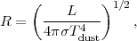(27)

and scaling to ULIRG luminosities, we obtain

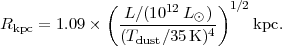(28)

This effective radius is the overall size of the optically-thick region emitting the FIR luminosity. In the event that the emission is optically thin, then the estimates from Equation 8.28 are of course lower limits. (In Section 8.2.9 optically-thick, radiative transfer modelling of the dust emission for a r^-1 dust density distribution is presented. Figure 8.15 shows the effective radius and dust temperature for the emitting region producing the majority of the emergent flux - for comparison with Equation 8.28.)

For local ULIRGs the typical FIR colour temperatures are ~ 50 K so the IR emission radius is ~ 500 pc for 10¹² L. This estimate is similar to the overall size of the central concentration in Arp 220 (see below), indicating that the optically thick assumption is not unreasonable. The most luminous SMGs observed at high redshift can have L_IR > 10¹³ L; for these sources, the emission must come from galactic-scale regions, not just a compact nucleus.

For the Milky Way the FIR luminosity is ~ 10¹⁰ L and the mean dust temperature ~ 30-35 K; the effective emitting radius from Equation 8.28 is ~ 100 pc. However, this emission clearly originates from a large number of separate clouds, and the mean size of each must be n_cloud^1/2 times smaller. For example, if the Galactic emission is assumed to be contributed by ~ 400 IR-luminous GMCs, then the effective size of the IR-dominant region in each would be ~ 5 pc.

8.2.8. Luminosity and SFR estimates from submm continuum

Estimating the FIR luminosity (and hence the SFR) from measurements on the submm R-J tail is an extremely questionable procedure - this hasn't stopped observers from routinely doing it! As noted above the R-J flux provides a measure of the dust mass weighed linearly by T_d, but inferring a total bolometric luminosity requires knowing where the FIR peaks, and the fluxes near the peak. Observations near the SED peak can now be done using Herschel PACS (Photodetector Array Camera and Spectrometer) and SPIRE (Spectral and Photometric Imaging REceiver) but many of the SMGs are subject to source confusion at the SPIRE resolution. In the absence of direct observations at the SED peak, one must assume a dust temperature (30-50 K) and optical depth, perhaps based on the submm flux. For many of the SMGs, FIR luminosities in the range 10^13-14 L have been estimated, implying SFRs of several × 10³ M per yr (typically assuming T_d ~ 30-50 K) but such estimates must be extremely uncertain since the derived luminosity will vary approximately as T^4-5. Typical ISM masses of the SMGs derived from CO measurements or the submm continuum are ~ 1-3 × 10¹⁰ M, implying that the ISM will be used up in star formation in an implausibly short time of ~ 10⁷ yr.

Blain et al. (2003) attempted to derive empirically a scaling between the 850 µm flux and L_IR based on the apparent T_d from fitting the SEDs of local galaxies. Unfortunately, there is large scatter in the correlation. In fact, as we saw earlier, the notion of a single T_d is extremely shaky - both because there clearly is a range of temperatures and more importantly, the apparent T_d (derived from fitting near the FIR peak) is somewhat degenerate with the dust opacity (which also can cause an exponential fall-off to short wavelengths).

To summarise - it should be clear that one cannot constrain T_d without observations near the SED peak; and if one has such observations, it would be best to simply use them directly to estimate the luminosity. (Of course, if the observed source is at redshift z > 5, then the submm flux measurements are in fact probing near the restframe SED peak; they can then provide a decent luminosity estimate.) In the next section, we model the optically-thick dust sources in order to appreciate some of the systematics and the range of uncertainty.

8.2.9. Modelling optically-thick dust clouds

For internally-heated FIR sources, it is vital to appreciate that the sources have essentially two totally independent parameters: the luminosity L of the central heating source and the total mass of dust in the surrounding envelope - not much else matters! The character of the spectrum of the source (be it young stars or an AGN) makes little difference since the primary photons at short wavelength are absorbed in the innermost boundary layer of the dust envelope. The radius of this inner boundary is set by the radius at which the dust is heated to sublimation (see Section 8.2.2). The overall mass of dust of course determines the opacity and therefore the radius at which the IR radiation can escape, and thus the `effective dust temperature' which is observed. We will see below that the model SEDs of the FIR sources can be characterised by a single parameter - the luminosity-to-mass ratio, L/M, and thus the problem has, in essence, really just one independent variable as long as the source structure is simple (e.g., a single source with radial fall-off in density and no clumping). The compactness of the dust cloud is parametrised by a radial power law density distribution which can be varied but for the discussion below I adopt R^-1.

Using the temperature profiles derived above, I have computed emergent spectra for a source of central luminosity 10¹² L with overlying dust masses ranging from 10^7-9 M (i.e., total ISM masses ~ 100 times greater or 10^9-11 M). These parameters are directed towards ULIRGs and SMGs but the results can easily be scaled to lower- or higher-luminosity objects. As mentioned above, the critical model characteristic is the luminosity-to-mass ratio. For this modelling, the dust distribution is taken to vary as R^-1 but similar results are found with other reasonable power laws. The inner radius is taken at T_d = 1000 K, but this is, of course, not critical since the hot dust is covered by the overlying colder dust unless the cloud is optically thin at short wavelengths. The outer radius was taken at 2 kpc - this also is not critical since the dust is cold and optically thin to the secondary radiation at the largest radii.

Figure 8.13 shows the emergent specific luminosities ( L) for the models with different enveloping dust masses but constant overall luminosity. Here one clearly sees the effect of varying dust mass and opacity. The clouds of lower dust mass have non-exponential short-wavelength SEDs due to the lack of high dust extinction on the short-wavelength side of the SED peak, and hence the hotter dust in the interior is exposed to our view. This contrasts with the higher-mass clouds which show a peak shifted to relatively longer wavelength - due to the fact that dust extinction short of the peak precludes photons escaping from the hotter interior radii. Figure 8.13 also clearly demonstrates the anticipated correlation (see Section 8.2.6) between the flux on the long-wavelength R-J tail and the dust mass.

Figure 8.13. The IR SEDs of dust cloud models with 1012 L are shown for increasing masses of overlying dust and an r-1 density distribution. The dust heating is provided by both the central source and secondary photons from warm dust (see text). The peak shifts to longer wavelength as the dust opacity increases and the R-J tail rises linearly with dust mass.

To quantify some of the spectral characteristics, Fig. 8.14 shows the shift in the wavelength of peak emission (_peak, left panel) and the optical depth at _peak to the cloud surface (right panel) for the radial shell contributing most to the emergent luminosity. The right panel illustrates what was said earlier based on analytics - typically the opacity at the peak will be ~1 for a large range of overlying dust masses. Also, since the opacity must be ~1 at the peak, the wavelength of peak emission will be determined by both opacity and dust temperature in realistic models.

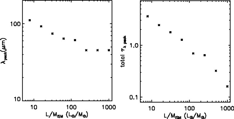Figure 8.14. The variation in the peak wavelength for L and the optical depth through the cloud at the peak wavelength are shown for varying L / MISM values with a density distribution of dust R-1. (Models run for power laws of 0, -1 and -2 exhibit similar behaviour as long as the clouds are optically thick.)

Figure 8.15 shows the radius and dust temperature at which the largest fraction of the overall luminosity escapes as a function of the luminosity-to-mass ratio. The total luminosity is of course spread over a broad range of radii except in the most optically thick models (low L / M_ISM values).

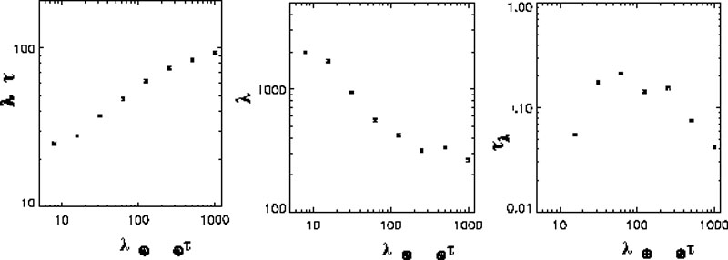Figure 8.15. Left and middle panels show the dust temperature and radius of the shell in the model producing the largest fraction of the overall luminosity for varying L / MISM values. The right panel shows the optical depth at the peak wavelength from this shell to the outer cloud surface - illustrating the fact that the emergent luminosity is produced at &tau ; 1. In most cases, the output luminosity is in fact spread over a fairly broad range of radii.

Figure 8.16 shows the ratio of total IR luminosity (at = 8-1000 µm) to the specific luminosity at = 850 µm (i.e., a point on the power-law R-J tail). It should be obvious from this figure that there is really no good single value for the conversion factor from submm flux density (_rest 150 µm) to total IR luminosity - these models all had the same total luminosity but varying dust masses. Thus it is impossible to reliably estimate the total FIR luminosity from R-J flux measurements unless there are additional constraints, for example on the luminosity-to-mass ratio or the ISM mass (e.g., from CO, or dynamical mass estimates). One simply must have measurements close to the IR SED peak.

Figure 8.16. The variation in the total IR luminosity to restframe 850 µm flux is shown for a range of L / MISM values, illustrating the impossibility of estimating the total IR luminosity from a single long-wavelength flux measurement.

There are also some limitations or lessons from this modelling. Most noteworthy is the polycyclic aromatic hydrocarbon (PAH) emission which arises from transiently heated small dust grains. This small grain component was included by calculating the UV-visual radiation energy density at each radius and inserting the PAH emission following Draine & Li (2001). These short-wavelength features require the emergence of flux from regions where the grains are hot. In sources showing such features, the dust obscuration must be clumpy, or multiple optically-thin and -thick sources must be contributing. To illustrate this possibility, Fig. 8.17 shows the effect of reducing the dust column in 5% of the surface area to a value 10% of the normal column density - the NIR/MIR becomes much stronger and the silicate feature appears in absorption.

Figure 8.17. Models with complete covering (dashed line) and with 5% of the area having extinction reduced to 10% and 1% of the complete covering model (solid line) are shown to illustrate that a slightly clumpy dust distribution is required to model the observed short-wavelength hot dust emission. Transient small grain heating is included by calculating the UV-visual radiation energy density at each radius and inserting the PAH emission following Draine & Li (2001).

The presence or absence of detectable PAH or silicates features depends on the covering fraction of the overlying optically-thick dust - their detection should not be taken as a reliable indicator of one mode of star formation (as done by Elbaz et al. 2011) or alteration of the grain abundances since their presence can depend simply on geometry and source non-uniformity.

8.2.10. Summary

We have developed a very simple model for the FIR emission which can be implemented for fast radiative transfer computations relevant to dust-embedded luminosity sources. There are several important conclusions:

1. For a central luminosity source, the dust temperature profile with radius can be modelled with very simply power laws: T_dust r^-0.42 for optically thin dust and T_dust r^-0.5 for optically thick dust. In a realistic source, it will be optically thin at the very innermost radius, optically thick at intermediate radii and optically thin at the outer radii; the temperature profile is then a piecewise fitting together of these two power laws.

2. To model the FIR sources, it is vital to recognise that there are two entirely independent parameters: the total luminosity and the mass of dust (and to a much lesser extent the radial profile of the dust distribution). Since the temperature profile scales with L, then most sources may be uniquely characterised by the ratio L / M_dust.

3. Using these temperature profiles, it is then straightforward and quick to calculate the emergent SED in the IR as a function of the ratio L / M_dust.

4. At the FIR peak, the emission is often optically thick (based on the steep fall-off in the SED to shorter wavelengths) but the optical depth will not be very large (i.e., _peak ~ 2-4) since otherwise the radiant luminosity would not be able to escape.

5. The effective dust temperature for the emergent luminosity can be determined approximately from the wavelength of the peak and then used to estimate an effective radius for the source.

6. Flux measurements on the R-J tail of the SED are uniquely capable for determination of the total dust mass (with a factor of two reliability) since the dust is optically thin. And if one can assume a dust-to-gas abundance ratio, such measures lead to quick and reliable estimates of a distant galaxy's total ISM content.

7. Determination of the total luminosity and hence the SFR requires observations near the peak at _rest ~ 100 µm; it can not be reliably estimated using a single long wavelength R-J flux measurement (as is often done for SMGs).

8. In optically-thick sources (as judged by the steep fall-off on the short side of the SED peak), the MIR emission at < 20 µm requires that the dust be somewhat clumped with incomplete covering in order to see the hot dust and the silicate and PAH features.