


As the methods of measuring of magnetic fields have been discussed widely in the literature, a short summary of the methods clarifies the present limitations.
2.1. Optical and far-infrared polarization
Elongated, rotating dust grains can be aligned with their major axis perpendicular to the field lines by paramagnetic alignment (Davis and Greenstein 1951) or, more efficiently, by radiative torque alignment (Hoang and Lazarian 2008). When the particles are observed with their major axis perpendicular to the line of sight (and the field is oriented in the same plane), the different extinction along the major and the minor axis leads to polarization, with the E-vectors pointing parallel to the field. This is the basis to measure magnetic fields with optical and near-infrared polarization, by observing individual stars or of diffuse starlight. Extinction is most efficient for grains of sizes similar to the wavelength. These small particles are aligned only in the medium between molecular clouds, not in the dense clouds themselves (Cho & Lazarian 2005).
The detailed physics of the alignment is complicated and depends on the
magnetic properties of the particles. The degree of polarization
p (in optical magnitudes) due to a volume element along the line
of sight  L is
given by
Ellis & Axon (1978):
L is
given by
Ellis & Axon (1978):
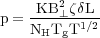 |
where T is the gas temperature, Tg is the grain
temperature, NH is the gas density,
 is the space density of
grains, B⊥ is the
magnetic field strength perpendicular to the line of sight.
is the space density of
grains, B⊥ is the
magnetic field strength perpendicular to the line of sight.
Light can also be polarized by scattering, a process unrelated to magnetic fields. This contamination is small when observing stars but needs to be subtracted from diffuse light, requiring multi-color measurements.
In the far-infrared (FIR) and submillimeter wavelength ranges, the emission of elongated dust grains is intrinsically polarized and scattered light is negligible. If the grains are again aligned perpendicular to the magnetic field lines, the E-vectors point perpendicular to the field. FIR polarimetry probes dust particles in the warm parts of molecular clouds, while sub-mm polarimetry probes grains with large sizes which are aligned also in the densest regions. The field strength can be crudely estimated from the velocity dispersion of the molecular gas along the line of sight and the dispersion of the polarization angles in the sky plane, the Chandrasekhar-Fermi method (Chandrasekhar & Fermi 1953), further developed for the case of a mixture of large-scale and turbulent fields by Hildebrand et al. (2009) and Houde et al. (2009).
Charged particles (mostly electrons) moving at relativistic speeds (cosmic rays) around magnetic fields lines on spiral trajectories generate electromagnetic waves. Cosmic rays in interstellar magnetic fields are the origin of the diffuse radio emission from the Milky Way (Fermi 1949; Kiepenheuer 1950). A single cosmic-ray electron of energy E (in GeV) in a magnetic field with a component perpendicular to the line of sight of strength B⊥ (in µG) emits a smooth spectrum with a maximum at the frequency:
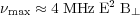 |
where B⊥ is the strength of the magnetic field component perpendicular to the line of sight. For particles with a continuous power spectrum of energies, the maximum contribution at a given frequency comes from electrons with about twice lower energy, so that max becomes about 4× larger.
The half-power lifetime of synchrotron-emitting cosmic-ray electrons is:
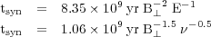 |
where B⊥ is measured in µG, E in GeV
and  in GHz.
The emissivity  from
cosmic-ray electrons with a power-law energy
spectrum in a volume with a magnetic field strength B⊥
is given by:
from
cosmic-ray electrons with a power-law energy
spectrum in a volume with a magnetic field strength B⊥
is given by:
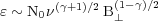 |
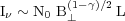
where is the frequency,
N0 is the density of cosmic-ray electrons per energy
interval,
 is the
spectral index of the power-law energy spectrum of the cosmic-ray
electrons (
≈ -2.8 for typical spectra in the interstellar medium of galaxies).
is the
spectral index of the power-law energy spectrum of the cosmic-ray
electrons (
≈ -2.8 for typical spectra in the interstellar medium of galaxies).
A source of size L along the pathlength has the intensity:
 |
A power-law energy spectrum of the cosmic-ray electrons with the
spectral index
leads to a power-law synchrotron spectrum I ~
 with the
spectral index
= ( + 1)
/ 2. The initial spectrum of young particles
injected by supernova remnants with
0
≈ -2.2 leads to an initial synchrotron spectrum with
0
≈ -0.6. These particles are released into the
interstellar medium. A stationary energy spectrum with continuous
injection and dominating synchrotron loss has
≈ -3.2 and
≈ -1.1. If the
cosmic-ray electrons escape from the galaxy faster than within the
synchrotron loss time, the stationary spectrum has
≈
(0
- ) ≈ -2.8 and
≈
(0 -
/2)
≈ -0.9, where
is the exponent of the
energy dependence of the electron
diffusion coefficient (D = D0 (E /
E0),
typically ≈ 0.6).
with the
spectral index
= ( + 1)
/ 2. The initial spectrum of young particles
injected by supernova remnants with
0
≈ -2.2 leads to an initial synchrotron spectrum with
0
≈ -0.6. These particles are released into the
interstellar medium. A stationary energy spectrum with continuous
injection and dominating synchrotron loss has
≈ -3.2 and
≈ -1.1. If the
cosmic-ray electrons escape from the galaxy faster than within the
synchrotron loss time, the stationary spectrum has
≈
(0
- ) ≈ -2.8 and
≈
(0 -
/2)
≈ -0.9, where
is the exponent of the
energy dependence of the electron
diffusion coefficient (D = D0 (E /
E0),
typically ≈ 0.6).
The energy densities of cosmic rays (mostly relativistic protons + electrons), of magnetic fields and of turbulent gas motions, averaged over a large volume of the interstellar medium and averaged over time, are comparable (energy equipartition):
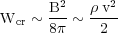 |
where Wcr is the energy density of cosmic rays,
B2 / 8 is the
energy density of the total magnetic field,
is the
energy density of the total magnetic field,
 v2 / 2 is the energy density of turbulent gas motions
with density
and
velocity dispersion v.
v2 / 2 is the energy density of turbulent gas motions
with density
and
velocity dispersion v.
On spatial scales smaller than the diffusion length of cosmic-ray electrons (typically a few 100 pc) and on time scales smaller than the acceleration time of cosmic rays (typically a few million years), energy equipartition is not valid.
Energy equipartition between cosmic rays and magnetic fields allows us to estimate the total magnetic field strength:
 |
This revised formula by
Beck & Krause (2005)
(see also
Arbutina et al. 2012)
is based on integrating the energy spectrum of the cosmic-ray
protons and assuming a ratio k between the number densities of
protons and electrons in the relevant energy range. The revised formula
may lead to significantly different field strengths than the classical
textbook formula which is based on integration over the radio frequency
spectrum. Note that the exponent of 2/7 given in the minimum-energy
formula in many textbooks is valid only for
= -2. The widely used
minimum-energy estimate of the field strength is smaller
than Beq by the factor ((1 -
) /
4)2/(5-), hence similar to Beq for
≈ -3.
The above formula is valid for steep spectra with
<
-2. For flatter
spectra, the integration over the energy spectrum of the cosmic rays
diverges and the calculation of Wcr has to be
restricted to a limited energy interval.
For electromagnetic particle acceleration mechanisms, the
proton/electron density ratio k for GeV particles is
≈ 40-100, which
directly follows from their different masses. (For an electron-positron
plasma, k = 0.) If energy losses of the electrons are significant,
e.g. in strong magnetic fields or far away from their places of origin,
k can be much larger, and the equipartition value is a lower limit of
the true field strength. (Due to the small exponent in the formula, the
dependence on the input parameters is weak, so that even large
uncertainties do not affect the result much.) On the other hand, the
nonlinear relation between
I and
B⊥ may lead to an overestimate of the
true field strength when using the equipartition estimate if strong
fluctuations in B occur within the observed volume. Another uncertainty
occurs if only a small volume of the galaxies is filled with magnetic
fields. Nevertheless, the equipartition assumption provides a reasonable
first-order estimate. Independent measurements of the field strength by
the Faraday effect in "magnetic arms" leads to similar values
(section 4.2). Furthermore, estimates of the
synchrotron loss time based on the
equipartition assumption can well explain the extent of radio halos
around galaxies seen edge-on (see
section 4.6). Finally, the magnetic
energy density based on the equipartition estimate is similar to that of
the turbulent gas motions (Fig. 20),
as expected from turbulent field amplification. Note that the
equipartition estimate still holds in starburst galaxies where secondary
electrons can contribute significantly
(Lacki & Beck 2013).
In our Galaxy the accuracy of the equipartition assumption can be tested
directly, because there is independent information about the energy
density and spectrum of local cosmic rays from in-situ measurements and
from -ray
data, which are emitted by the electrons via bremsstrahlung.
Combination with the radio synchrotron data yields a local strength of
the total field of ≈ 6 µG and ≈ 10
µG in the inner Galaxy. These values are
similar to those derived from energy equipartition. Combination of
radio and
-ray
data also yields field strengths similar to equipartition
in the Large Magellanic Cloud
(Mao et al. 2012)
and in the starburst region of M82
(Yoast-Hull et al. 2013).
Linear polarization is a distinct signature of synchrotron emission. The emission from a single electron gyrating in magnetic fields is elliptically polarized. An ensemble of electrons shows only very low circular polarization, but strong linear polarization with the plane of the E vector normal to the magnetic field direction. The intrinsic degree of linear polarization p is given by:
 |
Considering galactic radio emission with
≈ -2.8 a maximum of p0 = 74%
linear polarization is expected. In normal observing situations the
percentage polarization is reduced due to fluctuations of the magnetic
field orientation within the volume traced by the telescope beam
(section 2.3) or by Faraday depolarization
(section 2.4). The observed
degree of polarization is also smaller due to the contribution of
unpolarized thermal emission which may dominate in star-forming regions.
2.3. Magnetic field components
| Field component | Notation | Property | Observational signature |
| Total field | B2 = Bturb2 + Breq2 | 3D | Total synchrotron intensity, corrected for inclination |
| Total field perpendicular to the line of sight | B⊥2 = Bturb,⊥2 + Breq,⊥2 | 2D | Total synchrotron intensity |
| Turbulent field | Bturb2 = Biso2 + Baniso2 | 3D | Total synchrotron emission, partly polarized, corrected for inclination |
| Isotropic turbulent field perpendicular to the line of sight | Biso,⊥ | 2D | Unpolarized synchrotron intensity, beam depolarization, Faraday depolarization |
| Isotropic turbulent field along line of sight | Biso,|| | 1D | Faraday depolarization |
| Ordered field perpendicular to the line of sight | Bord,⊥2 = Baniso,⊥2 + Breq,⊥2 | 2D | Intensity and vectors of radio, optical, IR or submm polarization |
| Anisotropic turbulent field perpendicular to the line of sight | Baniso,⊥ | 2D | Intensity and vectors of radio, optical, IR or submm polarization, Faraday depolarization |
| Regular field perpendicular to the line of sight | Breg,⊥ | 2D | Intensity and vectors of radio, optical, IR or submm polarization |
| Regular field along line of sight | Breg,|| | 1D | Faraday rotation and depolarization, Zeeman effect |
The intensity of synchrotron emission is a measure of the number density of cosmic-ray electrons in the relevant energy range and of the strength of the total magnetic field component in the sky plane. Polarized emission emerges from ordered fields. As polarization "vectors" are ambiguous by 180°, they cannot distinguish regular (or coherent) fields with a constant direction within the telescope beam from anisotropic turbulent (or striated) fields, generated from isotropic turbulent magnetic fields by compression or shear of gas flows, which have a preferred orientation, but frequently reverse their direction on small scales. Unpolarized synchrotron emission indicates isotropic turbulent fields with random directions which have been amplified and tangled by turbulent gas flows.
Magnetic fields in galaxies preserve their direction only over the coherence scale, which can be determined by field tangling or by turbulence. If N is the number of cells with the size of the turbulence scale within the volume observed by the telescope beam and if the coherence length is constant, wavelength-independent depolarization occurs (Burn 1966):
 |
If the medium is pervaded by an isotropic turbulent field Bturb (unresolved field with randomly changing direction) plus an ordered field Bord (regular and/or anisotropic) which has a constant orientation in the volume observed by the telescope beam, it follows for constant density of cosmic-ray electrons:
 |
and for the equipartition case (Sokoloff et al. 1998):
 |
where q = Biso,⊥ / Bord,⊥ (components in the sky plane). This gives larger DP values (i.e. less depolarization) than for the former case.
2.4. Faraday rotation and Faraday depolarization
The linearly polarized radio wave is rotated by the Faraday effect in the passage through a magneto-ionic medium (Fig. 1). This effect gives us another method of studying magnetic fields — their regular component along the line of sight. The rotation angle induced in a polarized radio wave is given by:
 |
with  wavelength of
observation, ne thermal electron density,
B|| mean strength of the magnetic field component along the
line of sight, dl pathlength along the magnetic field.
wavelength of
observation, ne thermal electron density,
B|| mean strength of the magnetic field component along the
line of sight, dl pathlength along the magnetic field.
 |
Figure 1. Synchrotron emission and Faraday rotation |
and k is a constant (see below). In practice, the parameter Faraday Depth (FD) is used (Burn 1966):
 |
where
 |
with ne thermal electron density in cm-3, B|| mean strength of the magnetic field component along the line of sight in µGauss, L pathlength in parsec.
The observable quantity Rotation Measure (RM =

 /
2) is
identical to the physical quantity FD only in the rare cases when
is a linear function of
2. If the
rotating region is located in front of the
emitting region ("Faraday screen"), RM = FD. In case of a single
emitting and rotating region with a symmetric magnetic field profile, RM
≈ FD / 2 if Faraday depolarization (see below) is small.
/
2) is
identical to the physical quantity FD only in the rare cases when
is a linear function of
2. If the
rotating region is located in front of the
emitting region ("Faraday screen"), RM = FD. In case of a single
emitting and rotating region with a symmetric magnetic field profile, RM
≈ FD / 2 if Faraday depolarization (see below) is small.
As Faraday rotation angle is sensitive to the sign of the field direction, only regular fields give rise to Faraday rotation, while turbulent fields do not. For typical plasma densities and regular field strengths in the interstellar medium of galaxies, Faraday rotation becomes significant at wavelengths larger than a few centimeters. Only in the central regions of galaxies, Faraday rotation is strong already at 1-3 cm wavelengths. Measurements of the Faraday rotation angle from multi-wavelength observations allow determination the strength and direction of the regular field component along the line of sight. Its combination with the total intensity and the polarization pseudo-vectors yields in principle the three-dimensional picture of galactic magnetic fields and the three field components regular, anisotropic and turbulent.
By definition the regular magnetic fields point towards the observer when RM > 0. The quantity <neB||> is the average of the product (neB||) along the line of sight which generally is not equal to the product of the averages <ne><B||> if fluctuations in ne and B|| are correlated or anticorrelated. As a consequence, the field strength <B||> cannot be easily determined from RM even if additional information about <ne> is available, e.g. from pulsar dispersion measures (section 3.3).
Measurement of RM needs polarization observations in at least three
frequency channels with a large frequency separation in a frequency
range where Faraday depolarization is still small. In case of
strong Faraday depolarization (see below), the polarization angle
is no longer a linear
function of
2.
Large deviations from the
2 law can
also occur if several emitting and Faraday-rotating sources are
located within the volume traced by the telescope beam. In such cases,
the RM measured over a small wavelength range strongly fluctuates with
wavelength, and polarization data with many frequency channels
(spectro-polarimetry) are needed to allow application of RM Synthesis
(Brentjens & de Bruyn
2005).
RM Synthesis Fourier-transforms the complex polarization data from a limited part of the space into a data cube that provides at each point of the map a Faraday spectrum with FD as the third coordinate. The total span and the distribution of the frequency channels and the channel width define the resolution in the Faraday spectrum given by the width of the Rotation Measure Spread Function (RMSF), allowing the cleaning of the FD data cube, similar to cleaning of synthesis data from interferometric telescopes (Heald 2009). If the RMSF is sufficiently narrow, magnetic field reversals and turbulent fields can be identified in the Faraday spectrum (Frick et al. 2011; Bell et al. 2011; Beck et al. 2012). RM Synthesis is also able to separate FD components from distinct foreground and background regions and hence, in principle, to measure the 3D structure of the magnetized medium.
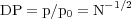
In a region containing cosmic-ray electrons, thermal electrons and purely regular magnetic fields, wavelength-dependent Faraday depolarization occurs because the polarization planes of waves from the far side of the emitting layer are more rotated than those from the near side. This effect is called differential Faraday rotation and is described (for one single layer with a symmetric distribution of thermal electron density and field strength along the line of sight) by (Burn 1966):
 |
where RM is the observed rotation measure, which is half of the total rotation measure through the whole layer. DP varies periodically with wavelength. With |RM| = 100 rad m-2 , typical for normal galaxies, DP has zero points at wavelengths of (12.5 √n) cm, where n = 1, 2, ... (Fig. 2). At each zero point the polarization angle jumps by 90°. Observing at a fixed wavelength hits zero points at certain values of the intrinsic RM, giving rise to depolarization canals along the level lines of RM. At wavelengths just below that of the first zero point in DP, only the central layer of the emitting region is observed, because the emission from the far side and that from the near side cancel (their rotation angles differ by 90°). Beyond the first zero point, only a small layer on the near side of the disk remains visible. Applying RM Synthesis to multichannel observations can recover the region as a broad component in the Faraday spectrum.
 |
Figure 2. Wavelength of maximum polarized emission for a synchrotron spectrum with spectral index = -0.9 and depolarization by differential Faraday rotation (Arshakian & Beck 2011) |
Turbulent fields also cause wavelength-dependent depolarization, called Faraday dispersion (Sokoloff et al. 1998). For an emitting and Faraday-rotating region (internal dispersion):
 |
where S = 2  RM2
4 .
RM2
4 .
RM2 is the dispersion in rotation
measure and depends on the turbulent field strength along the line of
sight, the turbulence scale, the thermal electron density, and the
pathlength through the medium. The main effect of Faraday dispersion is
that the interstellar medium becomes "optically thick" for polarized
radio emission beyond a wavelength, depending on
RM
(Fig. 3), and only a
front layer remains visible in polarized intensity. Galaxy halos and
intracluster media have typical values of
RM = 1-10 rad
m-2 while for galaxy disks typical values are
RM = 10-100
rad m-2 . Centers of galaxies
can have even higher dispersions. Fig. 3 shows
the optimum wavelength ranges to detect polarized emission for these
regions.
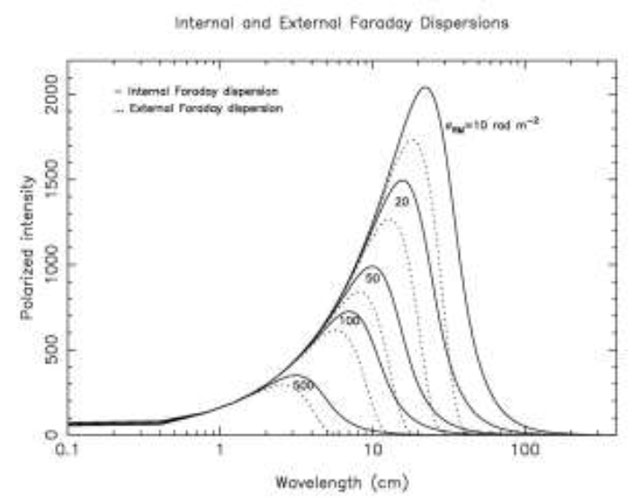 |
Figure 3. Wavelength of maximum polarized
emission for a synchrotron spectrum with spectral index
|
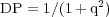
Regular fields in a non-emitting foreground Faraday screen do not depolarize, while turbulent fields do (external Faraday dispersion). For sources larger than the telescope beam:
 |
At long wavelengths S =
RM
2
(Tribble 1991).
Unresolved RM gradients within the beam also lead to
depolarization, similar to Faraday dispersion.
Faraday depolarization can also be classified as depth depolarization (differential Faraday rotation, Faraday dispersion along the line of sight) and beam depolarization (RM gradients, Faraday dispersion in the sky plane). Both types occur in emitting regions, while in non-emitting Faraday screens only beam depolarization occurs.
The Zeeman effect is the most direct method of remote sensing of
magnetic fields. It has been used in optical astronomy since the first
detection of magnetic fields in sunspots of the Sun. The radio detection
was first made in the HI line. In the presence of a magnetic field
B||
along the line of sight, the line at the frequency
0 is split into two
components (longitudinal Zeeman effect,
Fig. 4):
 |
where e, m and c are the usual physical constants. The two components are circularly polarized of the opposite sign. The frequency shift is minute, e.g. 2.8 MHz/Gauss for the HI line. More recent observation of the OH or H2O lines used the higher frequency shifts of these molecular line species (e.g. Heiles & Crutcher 2005). In magnetic fields perpendicular to the line of sight, two shifted lines together with the main unshifted line, all linearly polarized. This transversal Zeeman effect is much more difficult to observe and has not yet been detected in the interstellar medium.
 |
Figure 4. The longitudinal Zeeman effect, splitting of a line into two omponents with opposite circular polarization. |
2.6. Field origin and amplification
The origin of the first magnetic fields in the Universe is still a
mystery. The generation of the very first "seed" fields needs a
continuous separation of electric charges, e.g. by the Biermann
battery, the Weibel instability
(Lazar et al. 2009)
or fluctuations in the
intergalactic thermal plasma after the onset of reionization
(Schlickeiser 2012).
These may generate a seed field of ≤ 10-12 G in the
first galaxies or stars. A large-scale intergalactic field of
≤ 10-12 G may be generated in the early Universe
(Widrow 2002)
and could also serve as
a seed field in protogalaxies. This is consistent with the average
strength of intergalactic fields of ≥ 10-16 G, derived
from high-energy
-ray
observations with HESS and FERMI, assuming that the secondary particles
are deflected by the intergalactic fields
(Neronov & Vovk 2010).
However, such a large-scale primordial field is hard to maintain
because the galaxy rotates differentially, so that field lines get
strongly wound up, in contrast to the observations
(Shukurov 2005).
Moreover, a coherent large-scale field as observed e.g. in M31
cannot be explained by the primordial field model. The same is true for
kinematical models of field generation by induction in shearing and
compressing gas flows, which generate fields with a coherence length of
a few kiloparsecs and frequent reversals.
Magnetization of protogalaxies to ≥ 10-9 G could be achieved by field ejection from the first stars or the first black holes (Fig. 5), followed by dynamo action. The dynamo transfers mechanical into magnetic energy. It amplifies and/or orders a seed field. The small-scale or fluctuation dynamo does not need general rotation, only turbulent gas motions (Brandenburg & Subramanian 2005). The source of turbulence can be thermal virialization in protogalactic halos or supernovae in the disk or the magneto-rotational instability (MRI) (Rüdiger & Hollerbach 2004). Within less than 108 yr weak seed fields are amplified to the energy density level of turbulence and reach strengths of a few µG (Schleicher et al. 2010).
 |
Figure 5. Origin of seed fields in protogalaxies (Rees 2005). The last stage can be replaced by the small-scale dynamo. |
The "mean-field"
-
 dynamo is
driven by turbulent gas motions from supernova explosions or cosmic- ray
driven Parker loops ()
and by differential rotation
(),
plus magnetic diffusivity
(
dynamo is
driven by turbulent gas motions from supernova explosions or cosmic- ray
driven Parker loops ()
and by differential rotation
(),
plus magnetic diffusivity
( ) (e.g.
Parker 1979;
Ruzmaikin et al. 1988;
Beck et al. 1996).
It generates a large-scale ("mean") regular field from the
turbulent field in a typical spiral galaxy within a few 109
yr. If the small-scale dynamo already amplified turbulent fields of a
few µG in the
protogalaxy, the large-scale dynamo is needed only for the organization
of the field ("order out of chaos"). The field pattern is described by
modes of different azimuthal symmetry in the plane and vertical
symmetry or antisymmetry perpendicular to the plane. Several modes can
be excited in the same object. In almost spherical, rotating bodies like
stars, planets or galaxy halos, the strongest mode consists of a
toroidal field component with a sign reversal across the equatorial
plane (vertically antisymmetric or "odd" parity mode A0 with azimuthal
axisymmetry in the plane) and a poloidal field component of odd symmetry
with field lines crossing the equatorial plane
(Fig. 6). The halo mode
can also be oscillatory and reverse its parity with time (e.g. causing
the cycle of solar activity). The oscillation timescales (if any) are
very long for galaxies and cannot be determined by observations.
) (e.g.
Parker 1979;
Ruzmaikin et al. 1988;
Beck et al. 1996).
It generates a large-scale ("mean") regular field from the
turbulent field in a typical spiral galaxy within a few 109
yr. If the small-scale dynamo already amplified turbulent fields of a
few µG in the
protogalaxy, the large-scale dynamo is needed only for the organization
of the field ("order out of chaos"). The field pattern is described by
modes of different azimuthal symmetry in the plane and vertical
symmetry or antisymmetry perpendicular to the plane. Several modes can
be excited in the same object. In almost spherical, rotating bodies like
stars, planets or galaxy halos, the strongest mode consists of a
toroidal field component with a sign reversal across the equatorial
plane (vertically antisymmetric or "odd" parity mode A0 with azimuthal
axisymmetry in the plane) and a poloidal field component of odd symmetry
with field lines crossing the equatorial plane
(Fig. 6). The halo mode
can also be oscillatory and reverse its parity with time (e.g. causing
the cycle of solar activity). The oscillation timescales (if any) are
very long for galaxies and cannot be determined by observations.
 |
Figure 6. Poloidal field lines (a) and contours of constant toroidal field strength (b) for the simplest version of an odd-symmetry dipolar (top) and an even-symmetry quadrupolar (bottom) dynamo field (Stix 1975). More realistic dynamo fields can have many "poles". |
In flat, rotating objects like galaxy disks, the strongest mode of the
-
dynamo consists of a toroidal field component, which is symmetric with
respect to the equatorial plane and has the azimuthal symmetry of an
axisymmetric spiral in the disk without a sign reversal across the plane
(vertically symmetric or "even" parity mode S0), and a weaker poloidal
field co mponent of even symmetry with a reversal of the vertical field
component across the equatorial plane (Fig. 6).
The next higher
azimuthal mode is of bisymmetric spiral shape (even mode S1) with two
sign reversals in the plane, followed by more complicated modes. The
pitch angle of the spiral field depends mainly on the rotation curve of
the galaxy, the turbulent velocity and the scale height of the warm
diffuse gas
(Shukurov 2005).
The field in fast rotating galaxies has a
small pitch angle of about 10°, while slow differential rotation or
strong turbulence leads to larger pitch angles of 20° - 30°.
Enhanced supply of turbulent magnetic fields by the small-scale dynamo in spiral arms may result in a concentration of large-scale regular magnetic fields between the material arms (Moss et al. 2013), as observed in many galaxies (section 4.4). A similar result can be obtained by the inclusion of a fast outflow from spiral arms (Sur et al. 2007) or by introducing a relaxation time in the dynamo equation (Chamandy et al. 2013).
In principle, the halo and the disk of a galaxy may drive different dynamos and host different field modes. However, there is a tendency of "mode slaving", especially in case of outflows from the disk into the halo. The more dynamo-active region determines the global symmetry, so that the halo and disk field should have the same parity (Moss et al. 2010). This is confirmed in external galaxies (section 4.7), while our Milky Way seems to be different (section 3.5).
The ordering time scale of the
-
dynamo depends on
the size of the galaxy
(Arshakian et al. 2009).
Very large galaxies did not yet have
sufficient time to build up a fully coherent regular field and may still
host complicated field patterns, as often observed. The field ordering
may also be interrupted by tidal interactions or merging with another
galaxy, which may destroy the regular field and significantly delays the
development of coherent fields (section 5).
Strong star formation as the
result of a merger event or mass inflow amplifies the turbulent field
and can suppress the -
dynamo in a
galaxy if the total star-formation
rate is larger than about 20 solar masses per year. Continuous injection
of small- scale magnetic fields by the small-scale dynamo in turbulent
flows in star-forming regions may also decelerate the
-
dynamo and allow
initial field reversals to persist
(Moss et al. 2012).
The -
dynamo generates
large-scale helicity with a non-zero mean in each
hemisphere. As total helicity is a conserved quantity, small-scale
fields with opposite helicity are generated which suppress dynamo
action, unless these are removed from the system (e.g.
Vishniac et al. 2003).
Hence, outflow with a moderate velocity or diffusion is
essential for an effective
-
dynamo
(Sur et al. 2007).
This effect may
relate the efficiency of dynamo action to the star-formation rate in the
galaxy disk (section 4.6).
-
dynamo models
including outflows with moderate velocities can also generate X-shaped
fields
(Moss et al. 2010).
For fast outflows the advection time for the field becomes
smaller than the dynamo amplification time, so that the dynamo action is
no longer efficient.
There are several more unsolved problems with dynamo theory
(Vishniac et al. 2003).
The "mean - field" model is simplified because it assumes a
dynamical separation betwee n the small and the large scales. The
large-scale field is assumed to be smoothed by turbulent diffusion,
which requires fast and efficient field reconnection. One of the main
future tasks is to compute the "mean" quantities and from the
small-scale properties of the interstellar medium, which is only
possible with numerical modeling. MHD simulations of a dynamo driven by
the buoyancy of cosmic rays
(Hanasz et al. 2009)
and of a dynamo driven by supernovae
(Gressel et al. 2008;
Gent et al. 2013)
confirm the overall description of the
-
model. Improved
models with a spatial resolution of smaller than the turbulence scale,
hence ≈ 10 pc, should
include the whole rotating galaxy disk and the halo and consider all
relevant physical effects. The multiphase interstellar medium has also
to be taken into account
(de Avillez &
Breitschwerdt 2005).
Rapid progress in modeling galactic magnetic fields can be expected in
near future.
While the predictions of the
-
dynamo model have
been generally confirmed by present-day observations
(sections 4.3 and
4.6), the
primordial model of field amplification is less developed than the
dynamo model and is not supported by the data. A wound-up large-scale
seed field can generate only the even bisymmetric mode (S1) or the odd
dipolar mode (A0), both of which were not observed so far. On the other
hand, the number of galaxies with a well-determined field structure is
still limited (Appendix). Future radio
telescopes will be able to decide whether the dynamo or the primordial
model is valid, or whether a new model has to be developed.