2. BACKGROUND

The purpose of this long section is to introduce the concepts and mechanisms that are invoked in the main part of the review, which begins in Section 3. Note that I refer back to the various parts of this section where appropriate, so that those who start with the later sections can quickly locate a summary of the background that is assumed.

2.1. Galaxy formation

The current paradigm for galaxy formation is the CDM (Lambda Cold Dark Matter) model (Springel et al. 2006), which holds that galaxies form in dark matter halos whose distribution and properties were seeded by a Gaussian random field of tiny density fluctuations in the early Universe (Bardeen et al. 1986). Because the mean matter density was so close to the closure density in the early Universe, even very mild initial overdensities grew through self-gravity, and subclumps on all but the very largest scales were gravitationally bound together. In this epoch, few overdense regions were isolated from their neighbors, and the growth of structure was characterized by the development of a "cosmic web" of dense sheets, filaments and voids, that has been simulated with ever increasing precision (see Frenk & White 2012 for a recent review). During this phase, initially distinct collapse centers underwent a considerable degree of merging, giving each major overdensity a treelike origin as different leaves, branches and more major boughs join to the main density peak. Later, a little after redshift z ~ 1, some mysterious "dark energy", which has many of the properties of Einstein's cosmological constant, has caused the originally slowing universal expansion to reaccelerate (Riess et al. 1998; Perlmutter et al. 1999). Reacceleration increases the isolation of different pieces of the clustering hierarchy, reducing the later merging rate of halos and allowing galaxies to settle in a more dynamically quiescent period.

As the first collapses began, the mutual tidal stresses between the extended overdense regions impart some angular momentum about each collapse center. A dimensionless measure of the total angular momentum L is _L = L|E|^1/2 / GM^5/2, where E and M are the system's total energy and mass. Halos formed in hierarchical simulations are found to have a log-normal distribution of this parameter with a most probable value of _L,0 = 0.037 (Bullock et al. 2001). Stochastic hierarchical growth leads to a net angular momentum of a halo that varies in magnitude and direction both with distance from the point of highest density and over time.

The dynamical evolution just described is driven by the dark matter, popularly supposed to be some relic, weakly interacting particle that became nonrelativistic in the early Universe and is therefore described as "cold." It is believed (Hinshaw et al. 2013) to have a cosmic density more than 6 times that of the "baryonic" matter, comprised of the familiar protons, neutrons and electrons. The small mass fraction of hydrogen and helium, which combined from the primordial plasma to become neutral gas at z ~ 1100, is known to have subsequently reionized sometime around z ~ 10 (Larson et al. 2011) as the first objects dense enough to support thermonuclear reactions began to radiate.

Gas collected in overdense regions, either by cooling of shock heated material or through flows of cold gas accreted along filaments of the cosmic web, and spun up as it settled into rotationally supported disks at the centers of the dark matter halos. The on-going formation of stars in these gaseous disks gave rise to the galaxies we observe today. Numerical simulations of the galaxy formation process lack the dynamic range (Springel et al. 2006) to resolve the complicated gas physics of fragmentation, star formation, and the subsequent release of energy through supernovae (see Section 2.11). Thus the rate, efficiency, and precise location of star formation, described as "subgrid physics," is included in the simulations through rules that are both motivated by observational evidence and tuned to achieve the desired outcome. The difficulty that simulations have in making galaxylike objects with the properties we observe today is widely attributed to inadequacies in the implementation of star formation and feedback.

As halos continue to merge, the disks of stars that had begun to form in them are transformed into amorphous ellipsoidal components in the violently changing gravitational potential (Barnes & Hernquist 1992). Where some combination of shocks, supernovae, and active galactic nuclei has heated most remaining gas to very high temperatures, the merged remnants are believed to become the "red sequence" galaxies that have little gas that can cool and reconstitute an active star-forming disk. ¹ Where gas can cool and resettle, the ellipsoidal ball of stars becomes a spheroidal bulge at the center of a newly assembling disk that generally continues to grow. Disk galaxies that are actively forming stars are the "blue cloud" galaxies.

This current picture is widely accepted as broadly correct because it accounts for the distribution of galaxies throughout the Universe and some of their properties (Springel et al. 2006). Yet there are quite a number of important predictions of the model that seem to be inconsistent with known galaxy properties. Perhaps the foremost is that (1) many present-day galaxies lack the types of bulges produced by mergers (Shen et al. 2010; Kormendy et al. 2010), whereas the merging hierarchy of the model predicts substantial, dense bulges in most large galaxies. Other problems are (2) the central density of dark matter in the halos of galaxies today seem less than the models predict (Sellwood 2009; Kuzio de Naray & Spekkens 2011), (3) the number and properties of dwarf satellite galaxies surrounding each major galaxy seems inconsistent with what we observe (Boylan-Kolchin et al. 2012), (4) the old stars in galactic disks reside in a thinner layer that cannot have been stirred by a minor merger for a very long period (Wyse 2009), etc. See Silk & Mamon (2012) for a more detailed critique.

2.2. Relaxation time in the disks of galaxies

Except in the immediate neighborhood of a star, the gravitational attraction of nearby stars is generally negligible compared with that from the large-scale distribution of matter in a galaxy. While the argument that establishes this point can be found in many text books (e.g. Binney & Tremaine 2008 hereafter BT08), the usual derivation requires some modification for disk systems that is generally omitted even though it involves several nontrivial issues that are important both to the scattering of stars by mass clumps in the disk and to the proper interpretation of simulations, as noted elsewhere in this review.

2.2.1. Standard theory for spherical systems

A test particle moving at velocity v along a trajectory that passes a stationary field star of mass µ with impact parameter b is deflected by the attraction of the field star. For a distant passage, it acquires a transverse velocity component |v_⊥| 2Gµ / (bv) to first order (BT08 eq. 1.30). Encounters at impact parameters small enough to produce deflections where this approximation fails badly are negligibly rare and relaxation is driven by the cumulative effect of many small deflections.

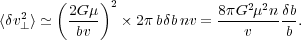
If the density of field stars is n per unit volume and uniform in 3D, the test particle encounters n = 2 b b nv stars per unit time with impact parameters between b and b + b. Assuming stars to have equal masses, each encounter at this impact parameter produces a randomly directed v_⊥ that will cause a mean square net deflection per unit time of

(1)

The total rate of deflection from all encounters is the integral over impact parameters, yielding

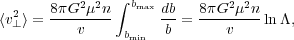(2)

where ln ≡ ln(b_max / b_min) is the Coulomb logarithm. Typically one chooses the lower limit to be the impact parameter of a close encounter, b_min 2Gµ / v², for which |v_⊥| is overestimated by the linear formula, while the upper limit is, say, the half mass or effective radius, R_e, of the stellar distribution beyond which the density decreases rapidly. The vagueness of these definitions is not of great significance to an estimate of the overall rate because we need only the logarithm of their ratio. The Coulomb logarithm implies equal contributions to the integrated deflection rate from every decade in impact parameter simply because the diminishing gravitational influence of more distant stars is exactly balanced by their increasing numbers.

Note that the first order deflections that give rise to this steadily increasing random energy come at the expense of second order reductions in the forward motion of the same particles that we have neglected (Hénon 1973). Thus the system does indeed conserve energy, as it must.

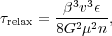
We define the relaxation time to be the time needed for < v_⊥² > v², where v is the typical velocity of a star. Thus

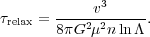(3)

To order of magnitude, a typical velocity v² ≈ GNµ / R_e, where N is the number of stars each of mean mass µ, yielding ≈ N. Defining the dynamical time to be _dyn = R_e / v and setting n ~ 3N / (4 R_e³), we have

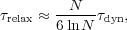(4)

which shows that the collisionless approximation is well satisfied in galaxies, which have 10⁸ N 10¹¹ stars. Including the effect of a smooth dark matter component in this estimate would increase the typical velocity, v, thereby further lengthening the relaxation time.

2.2.2. Applications to disk systems

This standard argument, however, assumed a pressure-supported quasispherical system in several places. Rybicki (1972) pointed out that the flattened geometry and organized streaming motion within disks affects the relaxation time in a number of important ways.

First, the assumption that the typical encounter velocity is comparable to the orbital speed v = (GNµ / R_e)^1/2 is clearly wrong; stars move past each other at the typical random speeds in the disk, say v with ~ 0.1, causing larger deflections and decreasing the time for < v_⊥² > ² v² by a factor ³.

Second, the distribution of scatterers is not uniform in 3D, as was implicitly assumed in eq. (1). Assuming a razor-thin disk changes the volume element from 2 v b b for 3D to 2v b in 2D, which changes the integrand in Eq. (2) to b^-2 and replaces the Coulomb logarithm by the factor (b_min^-1 - b_max^-1). In 2D therefore, relaxation is dominated by close encounters when the forces are Newtonian, and the system could never be collisionless.

Real galaxy disks are neither razor thin, nor spherical, so the spherical dependence applies at ranges up to the typical disk thickness z₀, beyond which the density of stars drops too quickly to make a significant further contribution to the relaxation rate. Thus we should use z₀ / b_min for disks.

Third, the local mass density is also higher, so that N ~ R_e² z₀ n. These three considerations shorten the relaxation time (Eq. 4) by the factor

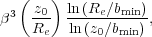(5)

or ~ 10^-4 for 0.1 and reasonable z₀ / R_e. Note that star-star encounters in galaxy disks remain unimportant, even with this large reduction in the relaxation time scale. But significant relaxation can occur in simulations of stellar disks, and the issues originally raised by Rybicki are of importance for scattering by clouds, as developed below.

A fourth consideration for disks is that the mass distribution is much less smooth than is the case in the bulk of pressure-supported galaxies. A galaxy disk generally contains massive star clusters and giant molecular clouds whose influence on the relaxation rate turns out to be non-negligible and also determines the shape of the equilibrium velocity ellipsoid (see Section 3.2.4).

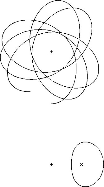Figure 1. An eccentric orbit in the midplane of an axisymmetric potential. The center of the potential is marked with a plus. The orbit is drawn in the inertial frame above and below in a frame that rotates with the guiding center, marked with a cross. Since the star conserves Lz, the motion around the epicycle is in the retrograde sense.

2.3. Stellar orbits in disks

While the above considerations should be borne in mind, it is nevertheless useful to regard the gravitational potential of a galaxy as a smooth function of position to a first approximation. If this assumption holds, the stellar component of a galaxy behaves as a collisionless fluid (BT08). I extend the discussion to include relaxation processes present in galaxy disks in Section 3.2.

A star, or test particle, moving in the symmetry plane (z = 0) of a steady axisymmetric potential (R, z) must conserve its specific energy E and specific angular momentum L_z about the symmetry axis (R = 0); these are the only two nontrivial integrals of motion when L_x = L_y = 0. In general, the orbit of a star is a rosette, as shown in Fig. 1, but when viewed from a frame rotating about the center of the galaxy at an angular frequency (lower panel), we see that the motion can be decomposed into a radial oscillation about a guiding center, which is marked with a cross, plus the uniform angular motion of the guiding center about the center with a period = 2 / . The guiding center radius R_g is where the radial acceleration of the particle passes through zero, i.e. where the central attraction matches the centripetal acceleration:

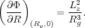(6)

For eccentric orbits, such as that shown, _c ≡ L_z / R_g², the angular frequency of circular motion for the same L_z. The radial oscillation is anharmonic and we simply define the radial frequency _R ≡ 2 / _R, where _R is the period of a full radial oscillation. In all realistic galactic potentials < _R < 2, and stars therefore make more than one, but less than two radial oscillations per orbit period. For near-circular orbits, → _c, and the radial oscillation becomes harmonic about the guiding center, with _R → , the Lindblad epicyclic frequency defined through

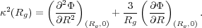(7)

Motion in the third dimension can also be oscillatory, with a well-defined period _z. When both the radial and vertical excursions are small, the vertical oscillation is decoupled from the in-plane motion, and has an angular frequency given by

(8)

Naturally, _z ≡ 2 / _z → in this limit.

In a general static, axisymmetric potential, the motion of most stars can be decomposed into three separate oscillations at the three different frequencies, _R, , and _z. Such orbits are described as regular orbits. However, there is a generally small fraction of irregular orbits, whose motion is more complicated and cannot be decomposed into three oscillations and another fraction that are truly chaotic.

In addition to the two classical integrals E and L_z, regular orbits respect a third, nonclassical integral. It is described as a nonclassical integral because it cannot be expressed as a simple function of the phase-space variables.

2.4. Action-angle variables

The formal clutter that usually accompanies any introduction to action-angle variables makes it hard to grasp what they really are and why they are useful. In an attempt to clarify these points, I here give a brief qualitative discussion, and refer the interested reader to BT08 for a more mathematical, but still not fully rigorous, treatment.

The 2D axisymmetric case, for which there are just two actions, is easiest to visualize and was illustrated already in Fig. 1. The azimuthal action J is simply the angular momentum, which is a measure of the size of the orbit or equivalently the radius of the guiding center (Eq. 6). The radial action J_R is a second conserved quantity that is a measure of the radial extent of the oscillation; thus J_R = 0 for a circular orbit and nonzero values can be calculated using Eq. (11). The orbit is uniquely determined by the values of the actions (J_R, J), which are an alternative pair of integrals to (E, L_z).

The doubly periodic motion is described by two angles w_R and w, which specify respectively the phase of the orbit around its epicycle and the phase of the guiding center around the galaxy center. One major advantage of this apparatus is that each angle variable increases at the constant rate w_i(t) = w_i(0) + t_i(E, L_z), even though the (R, ) coordinates of a star vary nonuniformly with time. ²

This approach becomes far more valuable when used to describe the 3D motion of a regular orbit, which respects three integrals. Even though one or more integrals cannot be expressed as simple functions of the phase-space variables in either Cartesian or polar coordinate systems, we can fully describe regular 3D motion in an arbitrary smooth potential using three actions that are conserved quantities, i.e. they are a set of integrals. The triply-periodic motion is described by three angles that again increase at uniform rates. The actions in an axisymmetric potential are J_R and J, the radial and azimuthal actions as for 2D, and J_z, which quantifies the up-and-down motion about the midplane. For each regular orbit, the three oscillation frequencies are _i = dw_i / dt = 2 / _i (Section 2.3), with i denoting any of the three cylindrical polar coordinates.

Not only do we now have a set of integrals and can describe the motion as the three angles increase in time at uniform rates, but these variables have two further advantages. The actions are the adiabatic invariants when the system is subject to slow changes, and the orbit is not close to a resonance. Finally, a more mathematical advantage is that perturbation theory is greatly simplified when using these variables (e.g. Section 3.5).

2.5. Orbital tori

Were motion confined to a plane, as for the 2D orbit shown in Fig. 1, the star would move in the 4D phase space (R, , v_r, v). However, because both E and L_z are conserved, the star's motion is confined to a 2D surface within the 4D phase space, since both velocity components v = L_z / R and v_R = {2[E - (R)] - (L_z / R)²}^1/2 are determined for every value of R, except for the sign ambiguity of v_R.

To see that the motion is confined to the surface a torus, imagine that we add to the rosette orbit shown in the upper panel, a third coordinate that is the star's radial velocity v_R, which is positive above the page and negative below. As the star moves forward in time from its pericentric distance, say, v_R first rises to a maximum height above the page as it crosses R_g, and then decreases to zero as it reaches its apocentric distance. Then v_R changes sign and the inward motion is below the page. As the star moves out and in, it also advances around the galactic center. Thus the motion in the 3D space of (R, , v_R) is confined to the surface of a torus in that space. It is impossible to visualize a fourth dimension, but while the speed v around the torus varies with R, it does so within a restricted range that does not alter the topology.

In 3D, stars move in a 6D phase space, and every conserved quantity, or isolating integral, confines its motion to a hyper-surface of one lower dimension. The regular orbit of a star that possesses three integrals is confined to the surface of a 3D hyper-torus in the 6D phase space, and again the motion within each dimension of the hyper-torus is an independent oscillation.

Fewer quantities are conserved for chaotic orbits, whose motion cannot be decomposed into three independent oscillations. For example, a star that moves chaotically is not confined to a 3D surface, but explores a 5D space if only E is conserved, which is typical in a nonaxisymmetric potential.

All three actions are quantities having the dimensions of angular momentum, and each is defined as the cross-sectional area of the appropriate slice through the star's orbit torus in 6D phase space, i.e.

(9)

where i labels a particular coordinate and the integral is around one complete loop in this slice through the torus. In an axisymmetric potential, J ≡ (2)^-1 ∫₀² vRd and, since the integrand Rv = L_z is a constant, we have J ≡ L_z, but Eq. (9) generally must be evaluated numerically for the other actions.

Since stars oscillate at differing frequencies in each of the three coordinate directions, one way to estimate the i-th action is to integrate the orbit and measure the area inside the closed curve delineated by the locus of points, or consequents, as the star crosses the 2D surface (x_i, x_i), known as the surface of section. McMillan & Binney (2008) described a superior method of "torus fitting" that yields all three actions simultaneously in an arbitrary potential.

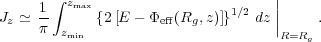
For those who find torus fitting intimidating, useful approximations can be obtained more easily for disk star orbits. We first assume axial symmetry, so that J = L_z, and write the energy of a star as

(10)

with the effective potential being _eff ≡ (R, z) + L_z² / (2R²). The approximation is to assume that the radial and vertical oscillations are decoupled, and that the radial action can be estimated from motion in the midplane as

(11)

The integration limits are the pericentric and apocentric values of R in the midplane, where the argument of the square root is zero. This integral is for half the radial period, and we drop the factor 2 in the denominator because the return half makes an equal contribution. Similarly,

(12)

These equations are exact for stars lacking vertical or radial oscillation, respectively, but in general they are slight overestimates since they assume that a star moving in 3D explores the full extent of the region that is energetically accessible, which is not quite the case when the orbit is integrated.

The epicyclic approximation for small-amplitude excursions assumes that both the radial and vertical oscillations are harmonic. If this is valid, J_R,epi = a² / 2, with a being the radial excursion of the star (Lynden-Bell & Kalnajs 1972) and J_z,epi = z_max² / 2. Since most stars in a disk have vertical excursions that take them outside the harmonic region of the disk potential well, J_z,epi should be avoided in favor of Eq. (12), which is readily evaluated.

2.6. Distribution function

The density of stars in the 6D phase space of position and velocity is given by a distribution function, f, hereafter DF. The DF for an equilibrium stellar system must be a function of the integrals only (Jeans theorem). The set of actions is a possible set of integrals, and the density of regular orbits could be written as f(J₁, J₂, J₃), but formally only if every possible orbit respects three integrals and there are no irregular or chaotic orbits.

For axisymmetric systems, if there were no third integral, the DF would be a function of the two classical integrals, E and L_z only. If this were true, the ratio of the second moments of the radial and vertical velocity components,

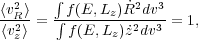(13)

as both and enter equally in E (Eq. 10). Since we observe that _R ≠ _z, we conclude that large parts of phase space of disks are regular and the effective DF must depend upon three integrals.

A few analytic expressions for DFs are known for 2D disks, but because the possible third integral is not a simple function of the phase-space coordinates, the development of analytic three-integral DFs for realistic flattened disks (e.g. Binney 2010) is much more difficult.

2.7. Nonaxisymmetric disturbances

Consider the potential of a small-amplitude disturbance in the z = 0 midplane that is the real part of

(14)

This potential has the following properties: it varies sinusoidally with the azimuthal coordinate , it is m-fold rotationally symmetric (e.g., m = 2 for a bi-symmetric spiral or bar), it rotates about the z-axis at the angular rate _p = ℜ() / m which is described as the pattern speed, and grows exponentially at the rate = ℑ(). The complex function (R) describes the radial variation of the amplitude and phase of the perturbation.

The density distribution that gives rise to this disturbance potential is not easily computed. Generally, Poisson's equation requires the potential spiral to be less tightly wound than the density spiral, and the phase relation between the density and potential therefore varies systematically with radius. The density and potential are in phase when the tight-winding (or WKB) approximation is employed, but spirals in galaxies are sufficiently open that this approximation gives only a rough guide to the dynamics of real spirals.

2.8. Resonances

Stars orbiting in the midplane of an almost axisymmetric galaxy are in resonance with a weak nonaxisymmetric disturbance of the form (14) when

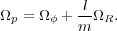(15)

The unperturbed orbit frequencies of the stars are defined in Section 2.3 and l is a signed integer. Equation (15) is satisfied for l = 0 when the guiding center of a star rotates synchronously with the disturbance, which is described as the corotation resonance. When l = ± 1, Eq. (15) defines the locations of the Lindblad resonances, which arise because the Doppler shifted frequency at which the star encounters the wave m| - _p| is equal to its unforced frequency of radial oscillation _R, or for nearly circular orbits. Interior to corotation, the stars overtake the wave, and l = -1 at the inner Lindblad resonance (ILR). Outside corotation, the stars are overtaken by the wave, and the outer Lindblad resonance (OLR) occurs where l = +1. Resonances for larger values of |l|, if they occur at all, are generally of little dynamical interest, since spiral patterns can exist only between the Lindblad resonances; a steady perturbing potential does not elicit a supporting response from the stars outside this radial range.

Ultraharmonic resonances arise where Eq. (15) is satisfied for l = ± 1 and m replaced by 2m. At these resonances, which are closer to corotation than are the Lindblad resonances, the star completes two radial oscillations as it moves between wave-crests. Yet higher-order resonances exist for larger integral numbers of radial oscillations; they are located still closer to corotation as stars drift ever more slowly relative to the pattern. Ultraharmonic resonances are dynamically unimportant in linear perturbation theory, but their nonlinear generalizations do play a role in finite-amplitude perturbations, especially bars (Section 5).

Vertical resonances will occur where the Doppler shifted frequency

(16)

with n being a signed integer; the n = 0 case (corotation) is of no special significance for vertical motion. In the epicycle approximation, _z → , which is a higher frequency in the massive part of the disk than is . Therefore, the n = ± 1 vertical resonances are farther from corotation than are the Lindblad resonances. In linear perturbation theory, spiral perturbations do not extend beyond the Lindblad resonances, making these vertical resonances uninteresting because the perturbation potential is tiny there. However, it should be noted that the effective vertical frequency _z ≡ 2 / _z can be much smaller than for stars with vertical excursions extending well outside the region where the potential is approximately harmonic, and such stars could, in principle, experience a vertical resonance.

Linear perturbation theory holds even at resonances for small-amplitude disturbances that grow exponentially, for then the resonances have a Lorentzian width determined by the growth rate. However, it breaks down for stars in resonance with a steady, or slowly growing, perturbation. Stars can be trapped by the resonance, and the size of the trapped region in phase space increases with the amplitude of the perturbing potential.

2.9. Local stability

The problem of computing the gravitational potential of an arbitrary spiral disturbance is one reason that the global normal modes of a stellar disk cannot be computed in a straightforward manner (Kalnajs 1977; Jalali 2007, BT08). While a WKB (local) approach, in which the local spatial variation of the disturbance can be approximated as part of a plane wave, is generally a poor approximation, results obtained using it do give some indication of the global behavior.

Toomre (1964) used this approximation to show that axisymmetric oscillations in a razor-thin disk of surface density are stabilized by rotation on scales

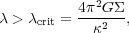(17)

where is the epicyclic frequency defined in Eq. (7). In the complete absence of random motion, a disk is unstable to gravitational clumping into rings on all scales smaller than _crit. Physically, _crit decreases with increasing because stars are held more tightly to their guiding center radii. The value of _crit ≈ 6 kpc in the solar neighborhood, or three fourths of the Sun's distance from the Galactic center, indicating that the WKB approximation is indeed stretched.

Random motions of the stars prevent gravitational instabilities when the disturbance disperses more rapidly than it grows. The tendency of random motions to provide stability on small scales while rotation suppresses instability on large scales, led Toomre to the following celebrated local stability criterion: if the stellar radial velocities have a Gaussian distribution with spread _R, then the system is axisymmetrically stable on all scales if

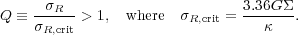(18)

Adopting solar neighborhood values, we find _{R, crit} ≈ 20 km s^-1. In a razor-thin, isothermal gas disk _R is replaced by the sound speed c_s and the constant 3.36 is replaced by . The constant is also slightly reduced in finitely thick disks since the destabilizing gravitational forces are diluted by the vertical spread of matter (e.g. Romeo 1992). The local stability of combined gas and stellar disks was calculated by Rafikov (2001), while Romeo & Wiegert (2011) offer an approximate formula for Q in thickened two-component disks. Global axisymmetric stability may be guaranteed if the disk is locally stable everywhere (Kalnajs 1976).

It cannot be emphasized too strongly that criterion (18) is for local axisymmetric stability only, and that disks that meet this criterion can still be unstable to nonaxisymmetric modes. In fact, no general criterion for nonaxisymmetric stability is known.

Local nonaxisymmetric stability was investigated by Goldreich & Lynden-Bell (1965) and by Julian & Toomre (1966), who independently discovered the process of swing-amplification. Figure 2, from a global calculation due to Toomre (1981), illustrates the fate of an arbitrary input leading spiral inserted by hand and given a pattern speed so that it is localized near the ILR. In this linearly stable, Q = 1.5 disk, the disturbance initially propagates away from the ILR and unwinds due to the differential rotation until it "swings" from leading to trailing. The disturbance is amplified by a large factor during this period when it is least wound because rotational support, which is a critical part of axisymmetric stability, is compromised briefly. The disturbance propagates radially at the group velocity (Toomre 1969), which is away from corotation for trailing waves, and the inner part returns toward the ILR. The part of the disturbance outside corotation fades quickly as it spreads over a wider area, while the opposite behavior affects the inner part until it is gradually absorbed by wave-particle interactions as it approaches the resonance. Thus the whole episode is a transient response that, to first order, causes no lasting change to the disk, although there are second order changes.

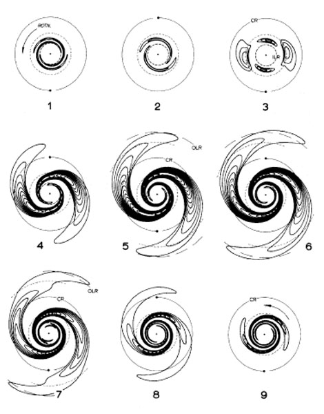Figure 2. The time evolution of an input leading wave packet in the half-mass Mestel disk. The unit of time is half a circular orbit period at the radius marked corotation. From Toomre 1981.

The amplification of a wave packet at corotation can be calculated in a variety of local approximations (Toomre 1981), while Drury (1980) computed the relationship between a continuous wave train incident on corotation and the super-reflected and transmitted waves. In the notation of Julian & Toomre (1966), the most important parameter is

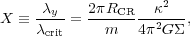(19)

where _y is the wavelength of the disturbance with angular periodicity m around the corotation circle of radius R_CR. For a flat rotation curve, amplification is significant for 1 X 3 and is strongest for an unwrapped wavelength that is about twice _crit. If the rotation curve declines, amplification extends to larger values of X and, conversely, it is confined to smaller X values in rising cases. Of course, the range of X for strong amplification shrinks to zero in the absence of shear (uniform rotation).

The amplification factor also decreases rapidly with increasing Q (Eq. 18). The reflected wave can be 100 times as strong as the incident wave for X 2 and Q 1.2, but only a few times greater when Q 2.

Notice that X ∝ (m)^-1, implying that for a fixed radius and rotation curve, amplification will be strong for higher m values when the disk surface density is low – i.e. we expect bisymmetric spirals in heavy disks and multi-arm spirals in strongly submaximal disks (Sellwood & Carlberg 1984). Thus the number of spiral arms in a galaxy could be an indicator of the relative contribution of the disk to the total central attraction (Athanassoula et al. 1987). This argument should not be applied to flocculent galaxies (Elmegreen & Elmegreen 1982), which have many small arm fragments, where the small spatial scale of the arms probably indicates that the responsive part of the disk is a low-mass component that has become dynamically decoupled from a hotter, underlying stellar disk.

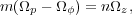
2.10. Angular momentum changes

The response of the stars to a weak potential perturbation is most easily calculated in action-angle variables (Lynden-Bell & Kalnajs 1972; Dekker 1976; Carlberg & Sellwood 1985; Binney & Lacey 1988). Lynden-Bell & Kalnajs (1972) showed that the first order changes in the angular momenta of stars average to zero everywhere. However, to second order, the rate of change in angular momentum of a group of stars is

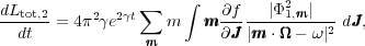(20)

plus a boundary term. Here the ranges of integration are unperturbed angular momenta L_{z, 1} ≤ J ≤ L_{z, 2} and radial action 0 ≤ J_R ≤ ∞. The _l,m are Fourier coefficients of the perturbing potential ₁ (Eq. 14), m = (l, m), J = (J_R, J), etc. Resonant denominators arise in Eq. (20) where m ⋅ = ℜ() (the same condition as Eq. 15), which pick out important locations in phase space where substantial changes take place. Note that the magnitude of each m-term depends on the gradient of the DF with rrespect to the actions at that resonance; thus the net change depends on the imbalance between those stars that lose on one side of the resonance compared with those that gain on the other side.

Generally, we expect f to be a decreasing function of all the actions in any reasonable galaxy; i.e. for a given L_z, there are more stars with small J_R and J_z and f falls off steeply with increasing values of either of these actions. Also the density of disk stars generally rises toward the center, and therefore f rises with decreasing J ≡ L_z, which is usually the shallowest of the three gradients.

A self-excited spiral involves no external torque, and this expression must therefore integrate to zero over the whole disk. However, Lynden-Bell & Kalnajs (1972) showed that the mean angular momenta of stars inward of corotation is lowered, and those outward are raised, by the growth of the disturbance. This feature allows a mode to extract energy from the gravitational potential well of the galaxy, enabling it to grow. Unfortunately, these angular momentum changes cannot be equated to the gravity torque between the misaligned density and potential because angular momentum can also be transported by a Reynolds-like advective stress (dubbed "lorry transport" by Lynden-Bell & Kalnajs 1972). The Reynolds stress is probably of minor importance in the vigorously growing modes that galaxies seem to support, but would be significant were quasi-steady spiral modes important.

2.11. Gas

The stars of a galaxy move on ballistic orbits that are affected only by gravitational forces. The fraction of the total baryonic mass contained in gas is generally less than 10% in large disk galaxies today. Over time, gas is converted into stars, but is replenished partly by returned material as massive stars end their lives, and also by on-going infall in spiral galaxies. The interstellar gas is collected into clouds, the diffuse ones being composed largely of neutral atomic hydrogen and helium with a sound speed c_s ~ 1.3 km s^-1, while dense molecular gas clouds are colder with c_s 0.5 km s^-1.

Typical orbital speeds in galaxies are 100 – 200 km/s, while typical velocity spreads of clouds about the mean orbital motion appear to have a lower bound of some 6 – 8 km s^-1, rising to twice this value in the bright, star-forming parts of disk galaxies. This supersonic turbulence (see Scalo & Elmegreen 2004 for a review) is maintained by a variety mechanisms, the most important of which is mechanical energy input through supernovae and, to a lesser extent, stellar winds (streams of particles accelerated from the surfaces of massive stars). When many massive stars are born at similar times in an exceptional burst of star formation, the ensuing rapid succession of supernovae can create a galactic wind that drives some of the gas out of the disk plane and perhaps, in the cases of small galaxies with shallow potential wells or young galaxies with high rates of star formation, right out of the galaxy. Large-scale dynamical phenomena, such as spiral activity, tidal interactions, and gas infall are other sources of turbulence.

The medium is also stirred by the magneto-rotational instability of weakly-magnetized differentially rotating fluid disks (Balbus & Hawley 1998; Sellwood & Balbus 1999), which maintains a lower level of trans-Alfvénic turbulence in parts of disks that have few young stars, and correspondingly few supernovae, where the dispersion remains about 6 km s^-1 (e.g. Dickey et al. 1990; Tamburro et al. 2009).

High spatial resolution simulations of this medium in small volumes (Stone et al. 1998; MacLow 1999) suggest that the magnetic field plays at most a secondary role in the dynamics of the gas clouds, which have a small filling factor. Collisions between clouds are highly supersonic and therefore strongly dissipative, with the thermal energy being radiated efficiently.

This complex medium is radiatively heated by stars to an extent that varies strongly with the proximity to clusters of hot young stars. It is also cooled radiatively through processes such as thermal bremsstrahlung, recombination lines from excited electronic states at rates that depend strongly on the fraction of heavy elements, various molecular rotational and vibrational transitions, and thermal emission from dust.

All these processes are intensely localized on spatial scales that are tiny compared with the overall size of a galaxy, and therefore well below the resolution limits of most simulations that attempt to model the formation and evolution of galaxies (see Sections 2.1 and 5.5).

However, despite the complicated microphysics of this heated, cooled, magnetized, and stirred multiphase medium, the crucial point is that turbulence cascades down to small scales where it is dissipated. Dissipation of random energy is the most important role of gas in the overall dynamics of the star plus gas disk. Galaxies lacking even a small fraction of mass in gas barely evolve. I emphasize the role of gas in appropriate places in this review.

2.12. Gravity softening in simulations

Computer simulations are powerful tools that have proved indispensible for unraveling the sometimes mystifying behavior of disk galaxies. Yet even with present-day computational power, simulations cannot routinely employ as many particles as there are stars in a galaxy. Thus some degree of smoothing of the mass distribution is needed, which also prevents strong accelerations during close encounters between the particles that would otherwise require adaptive time steps. Smoothing can be introduced directly through "softening" the interparticle force law at short range, or indirectly through the use of a grid, which similarly weakens the forces between particles on scales of the cell size (see the appendix of Sellwood & Merritt 1994). A third, but less general, method of smoothing is to determine forces from an expansion in some set of basis functions that is truncated at low order.

Note that shot noise from the particle distribution remains the most important limitation of simulations. The contribution of distant particles to the relaxation rate is unaffected by softening, which smooths fluctuations on only the smallest scales, and changes nothing in the formulae for relaxation but the value of the denominator of in the Coulomb logarithm (Section 2.2). Noise-driven density variations on larger scales can also excite non-negligible collective responses (Sellwood 1983; Toomre & Kalnajs 1991; Weinberg 1998).

2.12.1. 2D simulations

Simulating galaxy disks with the motion of particles confined to a plane has the obvious advantage of reduced computational cost over fully 3D simulations. The most appropriate gravity softening rule for 2D simulations is the Plummer law, for which the potential at distance d from a point mass is:

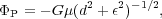(21)

where є is the gravitational softening length.

An advantage of the Plummer softening rule for this application is that it provides an approximate allowance for disk thickness, as follows. Convolution of Eq. (21) with the mass distribution of a razor-thin disk yields the exact Newtonian field in a plane offset by a vertical distance є from that containing the mass. In real finitely thick galaxy disks, the field everywhere is the sum of the Newtonian fields of the various mass elements spread in layers parallel to the midplane. The Newtonian forces experienced by the stars are therefore weaker than if the mass distribution were razor thin. Thus the value chosen for є in a 2D simulation should be closely related to the finite thickness of the disk (Romeo 1998).

Note that gravity softening weakens nonaxisymmetric instabilities (Sellwood 1983). Since the Newtonian potential of an arbitrary razor-thin mass distribution can be determined by expansion in Bessel functions (BT08, Section 2.6.2), the potential of each radial wavenumber, k, of the expansion decays away from the plane as exp(-|kz|). Further, since softened gravity is equivalent to sampling the field of a 2D mass sheet in a plane offset vertically by a distance є, the disturbance potential of each term is weaker by the factor exp(-|k|є). Hence instabilities are less vigorous. However, this weakening is physically realistic because softening provides an approximate allowance for the real finite thickness of galaxy disks as explained above.

To estimate the time for peculiar velocities to be randomized by encounters in 2D simulations, we replace Eq. (3) with

(22)

where n is now the number of particles per unit area, є = b_min and we assumed b_max^-1 ≪ b_min^-1. This formula, without the ³ factor, was already given by Hohl (1973). Setting N = R_e² n, with R_e being the half-mass radius of the disk, we find for 2D disks

(23)

This time is estimated for particles that interact with the forces derived from the potential of Eq. (21).

An advantage of computing forces through a cylindrical polar grid is that one can further smooth the mass distribution by restricting the sectoral harmonics m that contribute to the forces acting on each particle. The effect of restricting force terms to include only the range 0 ≤ m ≤ m_max is to replace each point particle by an azimuthally extended mass, providing some additional smoothing of the density distribution.

2.12.2. Simulations of thickened disks

In 3D simulations, the Plummer softening law (Eq. 21) has the undesirable property of weakening the interparticle force at all distances from the source particle, and a softening kernel that weakens forces only to a finite-range is greatly preferred. All that is needed for a serviceable softening kernel is that it should join smoothly to the Newtonian law at some distance є and yield an inter-particle force for d < є that smoothly approaches zero as d → 0. The precise form of the force at short-range should not matter because forces in a collisionless fluid are dominated by the distant mass distribution. Thus, if the behavior of the N-body system is to mimic that of a galaxy, its evolution should be insensitive to the adopted force law at short-range. Put another way, if the choice of the softening kernel affects the behavior, then the simulation is not collisionless.

Of its very nature, gravity softening limits the sharpness of forces that arise from steep density gradients. While the in-plane density distribution of galaxy disks varies on spatial scales that greatly exceed the values of є generally adopted, the disk mass is strongly confined to a plane. Unless the value of є ≪ z₀, the restoring force to the midplane will be weakened significantly, which has adverse consequences for the correct representation of buckling instabilities (see Section 5.4).

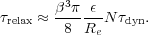
In quasispherical mass distributions, the relaxation rate is given by Eq. (4), with b_min = є in the Coulomb logarithm. Following the discussion in Section 2.2, we replace Eq. (4) for disks having a characteristic thickness, z₀, with

(24)

where the factor ³ is appropriate for the peculiar velocities to be randomized by encounters. For typical disk values of ~ 0.1 and z₀ / R_e ~ 0.1, this time is almost ~ 10⁴ times shorter than for quasispherical, pressure-supported systems with the same N (see also Sellwood 2013b).

¹ The terms "red sequence" and "blue cloud" refer to distinct groupings in the color-magnitude diagram for galaxies (e.g. Baldry et al. 2004) and reflect, more objectively, the distinction between early- and late-type galaxies already known to Hubble (e.g. Sandage 1961). Back.

² Lynden-Bell (1962) pointed out that while w_i(0) is a constant of the motion, it is a nonisolating integral, and therefore is of no importance to the overall structure of phase space. Back.