


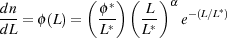
The evolving luminosity function is generally regarded as the best way to summarize the changing demographics of high-redshift galaxies. It is defined as the number of objects per unit comoving volume per unit luminosity, and the data are most often fitted to a Schechter function (Schechter 1976):
 |
(4) |
where ϕ* is the normalization density, L* is a characteristic luminosity, and α is the power-law slope at low luminosity, L. The faint-end slope, α, is usually negative (α ≃ -1.3 in the local Universe; e.g. Hammer et al. 2012) implying large numbers of faint galaxies.
In the high-redshift galaxy literature, the UV continuum luminosity function is usually presented in units of per absolute magnitude, M, rather than luminosity L, in which case, making the substitutions ϕ(M) dM = ϕ (L) d(-L) and M-M* = -2.5 log(L / L*), the Schechter function becomes
 |
(5) |
and this function is usually plotted in log space (i.e. log[ϕ(M)] vs. M).
The Schechter function can be regarded as simply one way of describing the basic shape of any luminosity function which displays a steepening above a characteristic luminosity L* (or below a characteristic absolute magnitude M*). Alternative functions, such as a double power-law can often also be fitted, and traditionally have been used in studies of the luminosity function of radio galaxies and quasars (e.g. Dunlop & Peacock 1990). Given good enough data, especially extending to the very faintest luminosities, such simple parameterizations of the luminosity function are expected to fail, but the Schechter function is more than adequate to describe the data currently available for galaxies at z ≥ 5. A recent and thorough overview of the range of approaches to determining and fitting luminosity functions, and the issues involved, can be found in Johnston (2011).
At the redshifts of interest here, the luminosity functions derived from optical to near-infrared observations are rest-frame ultraviolet luminosity functions. Continuum luminosity functions for LBGs are generally defined at λrest ≃ 1500 Å or λrest ≃ 1600 Å, while the luminosity functions derived for LAEs involve the integrated luminosity of the Lyman-α line. Because of the sparcity of the data at the highest redshifts, and the typical redshift accuracy of LBG selection, the evolution of the luminosity function is usually described in unit redshift intervals, although careful simulation work is required to calculate the volumes actually sampled by the filter-dependent selection techniques used to select LBGs and LAEs. Detailed simulations (involving input luminosities and sizes) are also required to estimate incompleteness corrections when the survey data are pushed towards the detection limit, and the form of these simulations can have a significant effect on the shape of the derived luminosity functions, especially at the faint end (as discussed by, for example, Grazian et al. 2011).
Different reported Schechter-function fits can sometimes exaggerate the discrepancies between the basic data gathered by different research groups. In particular, without good statistics and dynamic range, there can be severe degeneracies between ϕ*, L* and α, and very different values can be deduced for these parameters even when the basic statistics (e.g. integrated number of galaxies above the flux-density limit) are not very different (e.g. Robertson 2010).
This is an important point, because the luminosity-integral of the evolving luminosity function
 |
(6) |
(where Γ is the incomplete gamma function) is often used to estimate the evolution of average luminosity density as a function of redshift (from which the cosmic history of star-formation density and ionizing photons can be inferred; e.g. Robertson et al. 2010). For this reason care must be taken not to over-interpret the implications of extrapolating the fitted function (e.g. Su et al. 2011), especially when, as appears to be the case at very high redshift (see below), the faint-end slope is very steep. Formally, luminosity density diverges for α < -2 if the luminosity function is integrated to zero, but in practice the integral needs to be terminated at some appropriate faint luminosity (see section 6.1). The key point is that, for any steep faint-end slope even approaching α ≃ -2, the value of the integral depends critically on α and the adopted value of the faint-end luminosity cutoff (which, for obvious reasons, is still a matter of debate and could be a function of environment; Hammer et al. 2012).
At the bright end of the luminosity function the problem is generally not completeness but small-number statistics, and authors are often tempted to push their survey to produce a derived value for a brightest luminosity bin which depends on only a handful of objects. Given the small numbers, contamination by even rare populations (such as the brown dwarf stars discussed in section 3.1.3) can often be a problem at the bright end. An additional issue for a steeply-falling luminosity function is correcting for "Eddington bias", which tends to boost apparent average luminosity at the bright end. This again requires careful simulation to achieve a consistent solution. Finally it must be remembered that all luminosity functions are afflicted to some extent by cosmic variance (Sommerville et al. 2004), and ultimately high-redshift surveys need to cover sufficient area (helped by covering independent lines of sight) to offer a representative picture of the galaxy population at each epoch.
The comoving cosmological volumes sampled by various example LBG and LAE surveys at z ≃ 6 and z ≃ 7 are given for convenient comparison in Table 1.
| Survey Type | Redshift range | Area | Volume/Mpc3 | Example Reference |
| LBG WFCAM/VISTA | z = 5.5 - 6.5 | 1 deg2 | 10,000,00000 | McLure et al. (2009) |
| LAE Suprime-Cam(x4) | z = 5.7 ± 0.05 | 1 deg2 | 1,000,00000 | Ouchi et al. (2008) |
| LBG Suprime-Cam | z = 6.5 - 7.1 | 0.25 deg2 | 1,000,00000 | Ouchi et al. (2009) |
| LAE Suprime-Cam | z = 6.6 ± 0.05 | 0.25 deg2 | 200,00000 | Kashikawa et al. (2011) |
| LBG HUDF/WFC3 | z = 6.5 - 7.5 | 4.5 arcmin2 | 10,00000 | Oesch et al. (2010a) |
| LBG CANDELS/WFC300 | z = 6.5 - 7.5 | 0.2 deg2 | 1,500,00000 | Grogin et al. (2011) |
4.1. High-redshift evolution of the LBG luminosity function
The last ≃ 5 years have seen a rolling series of papers on the LBG UV luminosity function at z > 5, based purely on the ever-improving HST ACS, NICMOS, and now WFC3/IR deep imaging datasets (Bouwens et al. 2006, 2007, 2008, 2011b; Oesch et al. 2007, 2010a; Trenti et al. 2010)
In a complementary effort, McLure et al. (2009) focussed on determining the bright-end of the LBG luminosity function at z ≃ 5 and z ≃ 6 from ground-based data, before extending this work to z ≃ 7 and z ≃ 8 with WFC3/IR (McLure et al. 2010). In addition, the ground-based determination of the LBG luminosity function has recently been pushed out to z ≃ 7 by Ouchi et al. (2009) and Castellano et al. (2010a, b).
In general, the results of these various studies are in very good agreement. Specifically, McLure et al. (2009) combined their ground-based data on bright LBGs with the Bouwens et al. (2007) data on fainter HST-selected LBGs to determine the form of the UV luminosity function at z ≃ 5 and z ≃ 6, and derived Schechter-function parameter values in excellent agreement with Bouwens et al. (2007). The form and evolution of the LBG luminosity function deduced from this work is shown in the left-hand panel of Fig. 10, including the McLure et al. (2010) extension to z ≃ 7 and z ≃ 8. The simplest way to summarize these results is that the available data are consistent with α = -1.7 over the full redshift range z ≃ 5 - 7, and that the characteristic luminosity declines by a factor of two from z ≃ 5 (M* ≃ -20.7) to z ≃ 6 (M* ≃ -20.0) (as always one must caution this does not necessarily imply pure luminosity evolution of individual objects; see, for example, Stark et al. 2009).
 |
 |
Figure 10. The UV continuum LF of LBGs, and its high-redshift evolution. The left-hand panel shows the z ≃ 5 and z ≃ 6 LFs determined by McLure et al. (2009), along with the LFs at z ≃ 7 and z ≃ 8 determined by McLure et al. (2010) from the recent HST WFC3 imaging (the results obtained from a similar analysis by Bouwens et al. 2011b are summarized in Fig. 11). The right-hand panel demonstrates the extent of general agreement over the form and normalization of the UV LF at z ≃ 7 derived by different groups using both ground-based (Subaru & VLT) and HST WFC3/IR data. While the overall level of agreement is impressive, this plot also shows current tension over the true value of the faint-end slope, and the lack of information at the very bright end of the LF (courtesy R. McLure). |
|
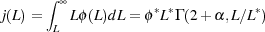
From z ≃ 6 to z ≃ 8 there is good agreement that the number density of LBGs continues to decline but uncertainties and degeneracies in the fitted Schechter-function parameters mean that it is currently hard to establish whether this evolution is better described as density or luminosity evolution. For example, McLure et al. (2010) concluded that the z ≃ 7 and z ≃ 8 luminosity functions are consistent with having the same overall shape at at z ≃ 6, but with ϕ* a factor of ≃ 2.5 and 5 lower, respectively. Ouchi et al. (2009) also concluded in favour of a drop in ϕ* between z ≃ 6 and z ≃ 7. Meanwhile, as shown in Fig. 11, the results of Bouwens et al. (2011b) appear to favour some level of continued luminosity evolution (perhaps also combined with a decline in ϕ* beyond z ≃ 6), but their best-fitting values for ϕ*, M* and α as a function of redshift are still consistent with the results of McLure et al. (2009, 2010) within current uncertainties (note that at z ≃ 8 current data do not really allow a meaningful Schechter-function fit).
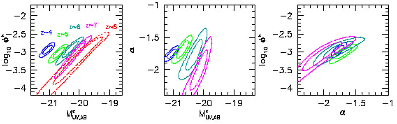 |
Figure 11. 68% and 95% likelihood contours on the model Schechter-function parameters derived by Bouwens et al. (2011b) from their determination of the UV (rest-frame ∼ 1700 Å) continuum LF at z ∼ 7 (magenta lines) and z ∼ 8 (dotted red lines). Also shown for comparison are the LF determinations at z ∼ 4 (blue lines), z∼5 (green lines), and z ∼ 6 (cyan lines) from Bouwens et al. (2007). No z ∼ 8 contours are shown in the center and right panels given the large uncertainties on the z ∼ 8 Schechter parameters. Fairly uniform evolution in the UV LF (left and middle panels) is seen as a function of redshift, although there remains significant degeneracy between ϕ* and M*. Most of the evolution in the LF appears to be in M* (particularly from z ∼ 7 to z ∼ 4). Within the current uncertainties, there is no evidence for evolution in ϕ* or α (rightmost panel)(courtesy R. Bouwens). |
There are, however, emerging (and potentially important) areas of tension. The right-hand panel of Fig. 10 shows the generally good level of agreement over the basic form of the LBG LF at z ≃ 7 (i.e. ϕ* ≃ 0.8 × 10⁻³ Mpc-3 and M* ≃ -20.1; Ouchi et al. 2009; McLure et al. 2010; Bouwens et al. 2011b), but also reveals issues at both the faint and bright ends (issues which we can hope will be resolved as the dataset on LBGs at z ≃ 7 - 8 continues to improve and grow).
At the faint end there is growing debate over the slope of the luminosity function. As summarized above, essentially all workers are in agreement that the faint-end slope, α, is steeper by z ≃ 5 than in the low-redshift Universe, where α ≃ -1.3. But recently, Bouwens et al. (2011b), pushing the new WFC3/IR to the limit with very small aperture photometry, have provided tentative evidence that the faint-end slope α may have steepened to α ≃ -2.0 by z ≃ 7. This "result" is illustrated in Fig. 10, which shows the confidence intervals on the Schechter parameter values deduced by Bouwens et al. (2011b) from z ≃ 4 to z ≃ 7. Clearly the data are still consistent with α = -1.7 over this entire redshift range, but given the luminosity function has definitely steepened between z ≃ 0 and z ≃ 5, further steepening by z ≃ 7 is certainly not implausible, and (as discussed above and in section 6) would have important implications for the integrated luminosity density, and hence for reionization. Fig. 11 also nicely illustrates the problems of degeneracies between the Schechter parameters; clearly it will be hard to pin down α without better constraints on ϕ* and M* which can only be provided by the larger-area surveys such as CANDELS and UltraVISTA (Robertson 2010). Another key issue is surface brightness bias. As discussed in detail by Grazian et al. (2011), because, for a given total luminosity, HST is better able to detect the most compact objects (especially in the very small (≃ 0.3-arcsec diameter) apertures adopted by Bouwens et al. 2011b), the estimated completeness of the WFC3/IR surveys at the faintest flux densities is strongly dependent on the assumed size distribution of the galaxy population. Thus, it appears that potentially all of any current disagreement over the faint-end slope at z ≃ 7 can be traced to different assumptions over galaxy sizes and hence different completeness corrections. Finally, there are of course the usual issues over cosmic variance, with the faintest points on the luminosity function being determined from the WFC3/IR survey of the HUDF which covers only ≃ 4 arcmin2. However, as discussed in detail by Bouwens et al. (2011b), it appears that large-scale structure uncertainties do not pose a very big problem for luminosity function determinations in the luminosity range -21 < M* < -18).
At the bright end, Fig. 10 illustrates that the problem is mainly lack of data, which in turn can be traced to a lack of large-area near-infrared surveys of sufficient depth and multi-frequency coverage. As discussed above, current ground-based surveys for LBGs at z ≃ 7 are limited to those undertaken by Ouchi et al. (2009) and Castellano et al. (2010a, b) and suffer from somewhat uncertain contamination due to lack of sufficiently deeper longer-wavelength data. Nevertheless, both Ouchi et al. (2009) and Castellano et al. (2010b) conclude that a decline in the number density of brighter LBGs between z ≃ 6 and z ≃ 7 is now established with better than 95% confidence, even allowing for cosmic variance (the contrary results of Capak et al. 2011 can be discounted for the reasons discussed in section 3.1.3). Significant further improvement in our knowledge of the bright end of the LBG luminosity function at z ≃ 7 and z ≃ 8 can be expected over the next ≃ 3 years, from CANDELS (Grogin et al. 2011), the WFC3/IR parallel programs (Trenti et al. 2011, 2012; Yan et al. 2011) and from UltraVISTA (McCracken et al. 2012; Bowler et al. 2012).
4.2. High-redshift evolution of the Lyman-α luminosity function
In contrast to the steady decline seen in the LBG ultraviolet continuum luminosity function at high redshift, there is little sign of any significant change in the Lyman-α luminosity function displayed by LAEs from z ≃ 3 to z ≃ 5.5. Indeed, as shown in Fig. 12, Ouchi et al. (2008) and Kashikawa et al. (2011) have presented evidence that the Lyman-α luminosity function displayed by LAEs selected via narrow-band imaging (and extensive spectroscopic follow-up) at z ≃ 5.7 is, within the uncertainties, essentially identical to that seen at z ≃ 3. Both studies were unable to constrain the faint-end slope of the Lyman-α luminosity function but, assuming α = -1.5, reported fiducial values for the other Schechter parameters at z = 5.7 of ϕ* ≃ 8 × 10⁻⁴ Mpc-3 and LLyα* = 7 × 1042 erg s-1.
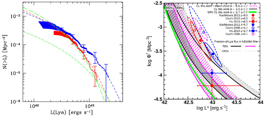 |
Figure 12. Current constraints on the Lyman-α LF at high redshift. The left-hand plot, taken from Kashikawa et al. (2011), shows a comparison of the cumulative Lyman-α LFs of LAEs at z = 5.7 (blue-shaded region) and at z = 6.5 (red-shaded region). The upper-edge of each shaded region is based on the assumption that all photometrically-selected candidates in the two SDF samples are indeed LAEs, while the lower-edge is derived purely on the spectroscopically-confirmed sample at each redshift. The short-dashed lines (red for z = 6.5 and blue for z = 5.7) show the fitted Schechter LFs assuming α = -1.5. For comparison, the green long-dashed line shows the Lyman-α LF at z = 6.5 determined from the larger area SXDS survey by Ouchi et al. (2010), and the green dot-dashed line shows the z = 6.5 Lyman-α LF determined by Hu et al. (2010) (courtesy N. Kashikawa). The right-hand plot, taken from Clément et al. (2012) summarizes our current knowledge (including some controversial disagreement) of ϕ* and L* for Schechter-function fits to the Lyman-α LF at z = 5.7 and z = 6.6 (again assuming α = -1.5), as well as attempting to set joint limits on these two parameters at z = 7.7 (see text in section 4.2 for details; courtesy B. Clément). |
Why the Lyman-α luminosity function should display different evolution to the LBG continuum luminosity function is a subject of considerable current interest. The relationship between LBGs and LAEs is discussed at more length in the next subsection (including the evolution of the ultraviolet continuum luminosity function of LAEs), but the key point to bear in mind here is that the evolution of the Lyman-α luminosity function inevitably reflects not just the evolution in the number density and luminosity of star-forming galaxies, but also cosmic evolution in the escape fraction of Lyman-α emission. This latter could, for example, be expected to increase with increasing redshift due to a decrease in average dust content, and/or at some point decrease with increasing redshift due to an increasingly neutral IGM.
Staying with the direct observations for now, at still higher redshifts the situation is somewhat controversial. Following Kashikawa et al. (2006), Ouchi et al. (2010) have extended the Subaru surveys of narrow-band selected LAEs at z ≃ 6.6 to the SXDS field. They conclude that there is a modest (≃ 20-30%) decline in the Lyman-α LF over the redshift interval z ≃ 5.7 - 6.6 (also shown in the left-hand panel of Fig. 12), and that this decline is best described as luminosity evolution, with LLyα* falling from ≃ 7 to ≃ 4.5 × 1042 erg s-1, while ϕ* remains essentially unchanged at ≃ 8 × 10⁻⁴ Mpc-3 (see right-hand panel of Fig. 12, again assuming α = -1.5).
The results from Ouchi et al. (2008; 2010) are based on large LAE samples but with only moderate levels of spectroscopic confirmation. These results have recently been contested by Hu et al. (2010). As summarized in the right-hand panel of Fig. 12, Hu et al. (2010) report a comparable value of L* at z ≃ 5.7, but ϕ* an order of magnitude lower. They then also report a modest drop in LAE number density by z ≃ 6.6, but conclude this is better described as density evolution (with ϕ* dropping by a factor of ≃ 2).
Also included in Fig. 12 are the latest results from Kashikawa et al. (2011), who used further spectroscopic follow-up to increase the percentage of spectroscopically confirmed LAEs in the SDF narrow-band selected samples of Taniguchi et al. (2005) and Shimasaku et al. (2006) to 70% at z ≃ 5.7 and 81% at z ≃ 6.6. The outcome of the resulting luminosity function reanalysis appears, at least at z ≃ 5.7, to offer some hope of resolving the situation, with Kashikawa et al. (2011) reporting a value for ϕ* somewhat lower than (but consistent with) the value derived by Ouchi et al. (2008), and at least closer to the ϕ* value reported by Hu et al. (2010). But at z ≃ 6.6 the results from Kashikawa et al. (2011) remain at odds with Hu et al. (2010), with ϕ* still an order of magnitude higher, and modest luminosity evolution since z ≃ 5.7 (if anything offset by slight positive evolution of ϕ*, resulting in any significant decline in number density being confined to the more luminous LAEs). Given the high spectroscopic confirmation rates in the new Kashikawa et al. (2011) samples, the claim advanced by Hu et al. (2010) that the previous Ouchi et al. (2008, 2010) and Kashikawa et al. (2006) studies were severely affected by high contamination rates in the narrow-band selected samples now seems untenable. Rather, it apears much more probable that the Hu et al. (2010) samples are either affected by incompleteness (and hence they have seriously under-estimated ϕ* for LAEs at high redshift), or that our knowledge of the Lyman-α luminosity function at z ≃ 6.6 is still severely confused by the affects of cosmic variance and/or patchy reionization (see, for example, Nakamura et al. 2011), an issue which is discussed further in section 5.5.
The recent work of Cassata et al. (2011), based on a pure spectroscopic sample of (mostly) serendipitous Lyman-α emitters found in deep VIMOS spectroscopic surveys with the VLT, also yields results consistent with an unchanging Lyman-α luminosity function from z ≃ 2 to z ≃ 6. In addition, their estimated values of ϕ* and LLyα* at z = 5-6 are in excellent agreement with those reported by Ouchi et al. (2008) at z ≃ 5.7. Interestingly, because the VIMOS spectroscopic surveys can probe to somewhat deeper Lyman-α luminosities than the narrow-band imaging surveys, this work has also provided useful constraints on the evolution of the faint-end slope, α, at least at moderate redshifts. Specifically, Cassata et al. (2011) conclude that α steepens from ≃ -1.6 at z ≃ 2.5 to α = -1.8 at z ≃ 4. Direct constraints at the highest redshifts remain somewhat unclear, but the clear implication is that, as for the LBG luminosity function, the faint-end slope is significantly steeper than α = -1.5 at z > 5 (and hence it is probably more appropriate to consider ϕ* and LLyα* values reported by authors assuming α = -1.7 or even α ≃ -2).
Finally, also shown in Fig. 12 are limits on the luminosity function parameter values at z ≃ 7.7 (albeit assuming α = -1.5), imposed by the failure of Clément et al. (2012) to detect any LAEs from deep HAWK-I VLT 1.06 µm narrow-band imaging of three 7.5 × 7.5 arcmin fields (probing a volume ∼ 2.5 × 10⁴ Mpc3). The ability of Clément et al. (2012) to draw crisp conclusions from this work is hampered by the confusion at z ≃ 6.6, with the above-mentioned different LFs of Ouchi et al. (2010), Hu et al. (2010) and Kashikawa et al. (2011) predicting 11.6, 2.5 and 13.7 objects respectively in the Hawk-I imaging (if the luminosity function remains unchanged at higher redshifts). Clément et al. (2012) conclude that an unchanged Lyman-α luminosity function can be excluded at ≃ 85% confidence, but that this confidence-level could rise towards ∼99% if one factors in significant quenching of IGM Lyman-α transmission due to a strong increase in the neutral Hydrogen fraction as we enter the epoch of reionization (an issue discussed further in the next subsection). However, the issue of whether or not the Lyman-α luminosity function really declines beyond z ≃ 7 undoubtedly remains controversial (e.g. Ota et al. 2010a; Tilvi et al. 2010; Hibon et al., 2010, 2011, 2012; Krug et al. 2012) and further planned surveys for LAEs at z ≥ 7 are needed to address this question (e.g. Nilsson et al. 2007).
The recent research literature in this field is littered with extensive and sometimes confusing discussions over the differences and similarities between the properties of LBGs and LAEs. In the end, however, the LAE population must be a subset of the LBG population, and the reported differences must be due to the biases (sometimes helpful) which are introduced by the different selection techniques. One key area of much current interest is to establish whether/how the fraction of LBGs which emit observable Lyman-α varies with cosmic epoch, because this has the potential to provide key information on the evolution of dust and gas in galaxies, and on the neutral hydrogen fraction in the IGM. There are a number of lines of attack being vigorously pursued, and I start by considering how we might reconcile the apparently very different high-redshift evolution of the Lyman-α and LBG ultraviolet luminosity functions (as summarized in the previous two subsections).
4.3.1. Comparison of the LBG UV and LAE Lyman-α luminosity functions
First, given the steady negative evolution of the LBG luminosity function from z ≃ 3 to z ≃ 6, and the apparently unchanging form and normalization of the Lyman-α luminosity function over this period, it seems reasonable to deduce that on average the fraction of Lyman-α photons emerging from star-forming galaxies relative to the observed continuum emission increases with increasing redshift out to at least z ≃ 6. Indeed Hayes et al. (2011) have used this comparison to deduce that the volume averaged Lyman-α escape fraction, fescLyα, grows according to fescLyα ∝ (1 + z)2.5 (normalized at ≃ 5% at z ≃ 2 through a comparison of the Lyman-α and H-α luminosity functions, currently feasible only at z ≃ 2). This result is shown in Fig. 13, which also shows that extrapolation of the fit to higher redshifts would imply fescLyα = 1 at z ≃ 11 in the absence of any new source of Lyman-α opacity, providing clear motivation for continuing the comparison of the Lyman-α and LBG continuum luminosity functions to higher redshift if at all possible (see below).
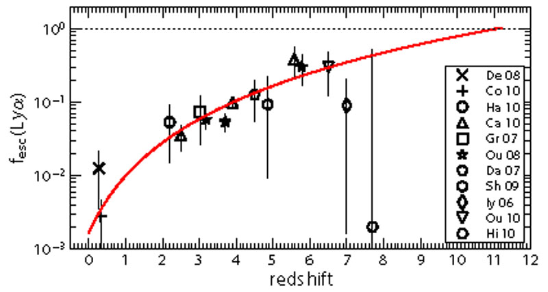 |
Figure 13. The redshift evolution of volume-averaged Lyman-α escape fraction, fescLyα, as deduced by Hayes et al. (2011), normalized to ≃ 5% at z ≃ 2 via comparison of the Lyman-α and H-α integrated luminosity functions, and deduced at higher redshifts by comparison of the Lyman-α and UV continuum luminosity functions discussed in sections 4.1 and 4.2. The solid red line shows the best-fitting power-law to points between redshift 0 and 6, which takes the form (1 + z)2.6, and appears to be a good representation of the observed points over this redshift range. It intersects with the fescLyα = 1 line (dotted) at redshift z = 11.1 (courtesy M. Hayes). |
4.3.2. The LAE UV continuum luminosity function
The italics in the preceding paragraph have been chosen with care, because we must proceed carefully. This is because the situation is confused by the fact that, for those galaxies selected as LAEs (via, for example, narrow-band imaging as discussed in detail above), the ratio of average Lyman-α emission to ultraviolet continuum emission apparently stays unchanged or even decreases with increasing redshift. We know this from studies of the ultraviolet continuum luminosity function of LAEs, which I have deliberately avoided discussing until now because there are complications in interpreting the UV continuum luminosity function of objects which have been selected primarily on the basis of the contrast between Lyman-α emission and UV continuum emission. Nevertheless, Ouchi et al. (2008) have convincingly shown that, while the Lyman-α luminosity function of LAEs holds steady between z ≃ 3 and z ≃ 5.7, the UV continuum luminosity function of the same objects actually grows with redshift, more than bucking the negative trend displayed by LBGs. Then, from z = 5.7 to z ≃ 6.6, as the Lyman-α luminosity function shows the first signs of gentle decline, Kashikawa et al. (2011) find that the UV continuum luminosity function of the LAEs stops increasing, but seems to hold steady. Another way of saying this is that the average equivalent width of Lyman-α emission in LAEs is constant or if anything slightly falling with increasing redshift. Indeed, Kashikawa et al. (2011) report that the median value of Lyman-α equivalent width falls from EWrest ≃ 90 Å at z ≃ 5.7 to EWrest ≃ 75 Å at z ≃ 6.6 although, interestingly, there is a more pronounced extreme EWrest tail in their highest-redshift sample.
Possible physical reasons for why this happens are discussed further below but, whatever the explanation, it is clear that the UV continuum luminosity function of LAEs cannot keep rising indefinitely, or it will at some point exceed the UV luminosity function of LBGs, which is impossible. Indeed, the two luminosity functions appear to virtually match at z ≃ 6. Specifically, as shown in Fig. 14, and as first demonstrated by Shimasaku et al. (2006), by z ≃ 6, LAE selection down to EWrest ≃ 20 Å recovers essentially all LBGs with M1500 < -20, to within a factor ≃ 2. It is thus no surprise that the UV luminosity function of LAEs must freeze or commence negative evolution somewhere between z ≃ 6 and z ≃ 7, as by then it must start to track (or fall faster than) the evolution of the (parent) LBG population.
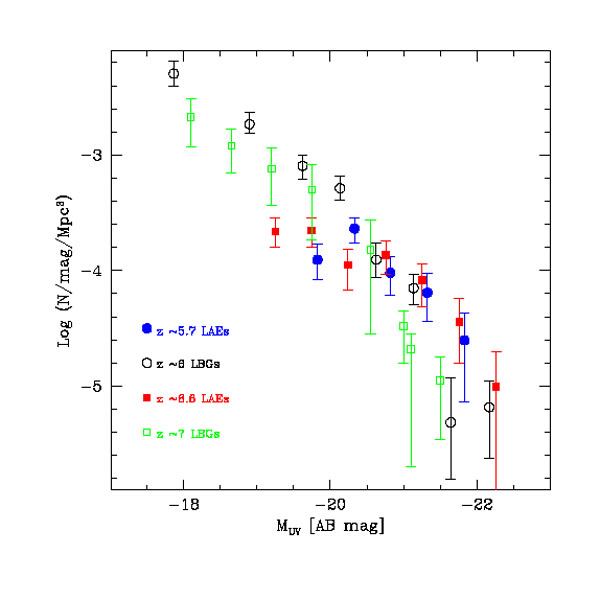 |
Figure 14. A comparison of the high-redshift UV continuum LFs of galaxies selected as LBGs and galaxies selected as LAEs. Shown here are the UV continuum LFs for LBGs at z ≃ 6 as determined by Bouwens et al. (2007), for LBGs at z ≃ 7 as determined by McLure et al. (2010), for LAEs at z ≃ 5.7 as determined by Shimasaku et al. (2006), and for LAEs at z ≃ 6.6 as as determined by Shimasaku et al. (2006). The LAE UV LFs become incomplete at MUV > -21 because of the limited depth of the ground-based broad-band imaging in the large Subaru survey fields (compared to the deeper HST data used to derive the LBG LFs). However, at brighter magnitudes the agreement between the z ≃ 6 LBG LF and the two LAE-derived LFs at z ≃ 5.7 and 6.6 is very good (courtesy P. Dayal). |
4.3.3. The prevalence of Lyman-α emission from LBGs
If this is true, then it must also follow that the fraction of LBGs which display Lyman-α emission with EWrest > 20 Å in follow-up spectroscopy must also rise from lower redshifts to near unity at z ≃ 6. There has been some controversy over this issue, but recent observations appear to confirm that this is indeed the case. First, Stark et al. (2011) have reported that, with increasing redshift, an increasing fraction of LBGs display strong Lyman-α emission such that, by z ≃ 6, over 50% of faint LBGs display Lyman-α with EWrest > 25 Å. Similarly high Lyman-α "success rates" have now been reported for more luminous (≃ 2 L*) LBGs at z ≃ 6 by Curtis-Lake et al. (2012) (Fig. 15), and by Jiang et al. (2011).
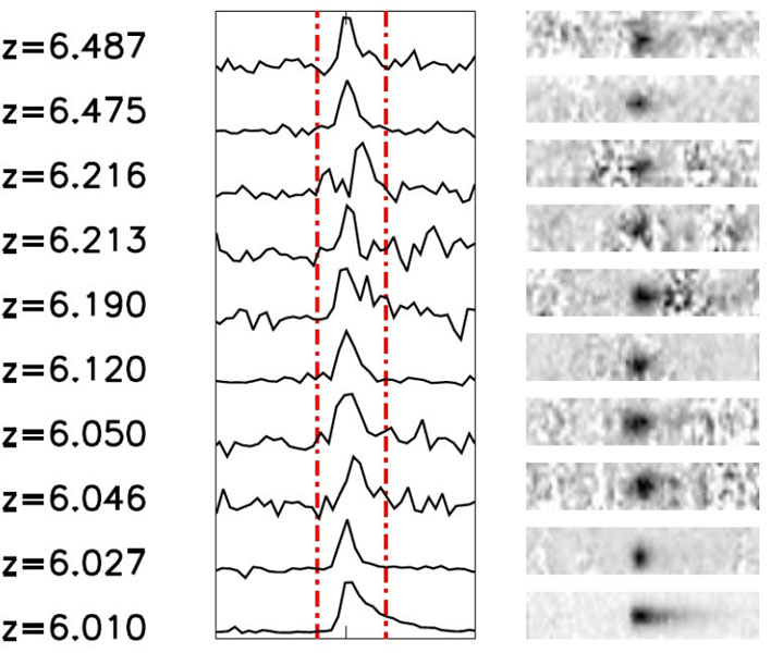 |
Figure 15. A high success rate in the detection of Lyman-α emission from bright LBGs at z = 6-6.5. VLT FORS2 spectra of 10 z > 6 LBGs selected from the UDS/SXDS field are shown; this represents 70% of the targetted high-redshift sample (Curtis-Lake et al. 2012). The extracted one-dimensional (1D) spectra are shown on the left, with the corresponding two-dimensional (2D) spectra on the right; Lyman-α emission (often obviously asymmetric) is clearly detected from all of these objects (courtesy E. Curtis-Lake). |
4.3.4. Reconciliation to z ≃ 6
It thus appears that the average volumetric increase in Lyman-α emission relative to ultraviolet continuum emission as summarized by Hayes et al. (2011) to produce Fig. 13 is due to an increase with redshift in the fraction of star-forming galaxies which emit at least some detectable Lyman-α emission rather than a systematic increase in the Lyman-α to continuum ratio of objects which are selected as LAEs at all epochs.
As already discussed above, one thing which is clear, and perhaps surprising, is that by z ≃ 6, narrow-band selection of LAEs from the wide-area Subaru surveys seems to be an excellent way of determining the bright end of the complete LBG UV luminosity function, indicating that the fraction of LBGs which display EWrest > 10 Å is approaching unity by this redshift. We stress that this is not the same as seeing all of the Lyman-α emission from the star-forming population; it is perfectly possible for virtually all the LBGs to emit enough Lyman-α to be detected in deep LAE surveys, while still having some way to go before the overall volume-average Lyman-α escape fraction could be regarded as approaching unity. Put another way, it is not unreasonable to conclude that the detection rate of bright LBGs in LAE surveys reaches 100% at z ≃ 6, while volume-averaged fescLyα as plotted in Fig. 13 has only reached ≃ 40-50%. As discussed below, there may be good astrophysical reasons why the volume-averaged fescLyα never reaches 100%.
Given that, at least for M1500 < -20, current LAE and LBG surveys appear to be seeing basically the same objects at z ≃ 6, it makes sense to consider what, if anything, can be deduced about the fainter end of the LBG UV luminosity function from those LAEs which are not detected in the continuum. As can be seen from Fig. 14, the ground-based imaging from which the LAE samples are selected, not unexpectedly runs out of steam at flux densities which correspond to M1500 ≃ -21 at z ≃ 6.6. But there still of course remain many (in fact the vast majority of) LAEs which have no significant continuum detections, and these objects are not only useful for the Lyman-α luminosity function, but potentially also carry information on the faint end of the LBG UV luminosity function. The question is of course how to extract this information. One could follow-up all the LAEs which are undetected in the ground-based broad imaging with HST WFC3/IR to determine their UV luminosities (i.e. M1500); this would undoubtedly yield many more detections allowing further extension of the UV continuum luminosity function of LAEs to fainter luminosities. However, this would still not overcome another incompleteness problem which is that, as narrow-band searches are limited not just by equivalent width, but also by basic Lyman-α luminosity, the subset of LBGs detectable in the LAE surveys becomes confined to those objects with increasingly extreme values of EWrest as we sample down to increasingly faint UV luminosities. Then, even with deep WFC3/IR follow-up of detectable LAEs, and even assuming all LBGs emit some Lyman-α, we would still be forced to infer the total number of faint LBGs by extrapolating from the observable extreme equivalent-width tail of the LAE/LBG population assuming an equivalent-width distribution appropriate for the luminosity and redshift in question.
This is difficult, and presents an especially severe problem at high-redshift, where our knowledge of Lyman-α equivalent-width distributions is confined to the highest luminosities. Nevertheless, Kashikawa et al. (2011) have attempted it, and discuss in detail how they tried to arrive at an appropriate equivalent-width distribution as a function of UV luminosity at z ≃ 6.6. A key issue is that it is difficult, if not impossible, to determine the UV continuum luminosity dependence of Lyman-α EWrest in the underlying LBG population from the equivalent-width distribution displayed by the narrow-band selected LAEs themselves, as this is in general completely dominated by the joint selection effects of Lyman-α luminosity and equivalent width. There has indeed been much controversy over this issue, with Nilsson et al. (2009) claiming that, at z ≃ 2-3 where LAE surveys display good dynamic range, there is no evidence for any UV luminosity dependence of the EWrest distribution, contradicting previous claims that there was a significant anti-correlation between EWrest and UV luminosity. Of course what is really required is complete spectroscopic follow-up of LBGs over a wide UV luminosity range, to determine the distribution of EWrest as a function of M1500, free from the biases introduced by LAE selection. This has been attempted by Stark et al. (2010, 2011), and it is the results of this work that Kashikawa et al. (2011) have employed to try to estimate the faint end of the LBG UV luminosity function at z ≃ 6 from the number counts of faint (but still extreme equivalent width) LAEs extracted from the narrow-band surveys. The problem with this is that even the state-of-the-art work of Stark et al. (2011) only really provides EWrest distributions in two luminosity bins at z ≃ 6, and the apparent luminosity dependence inferred from this work is called into some question by the success in Lyman-α detection in bright LBGs at z ≃ 6 by Curtis-Lake et al. (2012) and Jiang et al. (2011). Thus, at present, our understanding of the luminosity dependence of the Lyman-α EWrest distribution displayed by LBGs remains poor, and is virtually non-existent for LBGs with M1500 > -19 at z > 6.
Nevertheless, the experiment is of interest, and the resulting UV LF derived from the Lyman-α LF by Kashikawa et al. (2011) is more like a power-law than a Schechter function. Moreover, the implied faint-end slope is extremely steep; if a Schechter-function fit is enforced, α = -2.4 results, even though the UV LF was inferred from a Lyman-α Schechter function with α = -1.5, which is probably too flat. It is not yet clear what to make of this result, but it would appear that either the equivalent-width distribution of Lyman-α from faint LBGs is biased to even higher values than assumed (so that even extreme equivalent-width LAEs sample a larger fraction of the LBG population at faint M1500 than anticipated by Kashikawa et al. 2011), or the incompleteness in the faint LBG surveys has been under-estimated. This latter explanation seems unlikely given the already substantial incompleteness corrections made by Bouwens et al. (2011), but is not entirely impossible if LAEs pick up not just the compact LBGs seen in the HST surveys, but also a more extended population which is missed with HST but is uncovered by ground-based imaging (which is less prone to surface-brightness bias). This, however, also seems unlikely; while recent work has certainly demonstrated that the Lyman-α emission from high-redshift galaxies is often quite extended (e.g. Finkelstein et al. 2011; Steidel et al. 2011), consistent with theoretcial predictions (e.g. Zheng et al. 2011), all evidence suggests that the UV continuum emission from these same objects is at least as compact as LBGs at comparable redshifts (i.e. typically rh ≤ 1 kpc at z > 5; Cowie et al. 2011; Malhotra et al. 2012; Gronwall et al. 2011). The fact that, due to the complex radiative transfer of Lyman-α photons, the Lyman-α morphologies of young galaxies are expected to be complex and in general more extended than their continuum morphologies is supported by new observational studies of low-redshift Lyman-α emitting galaxies as illustrated in Fig. 16 (from the Lyman Alpha Reference Sample – LARS; HST Program GO12310). However, from the point of view of luminosity-function comparison, the key point is that while extended low-surface brightness Lyman-α emission might be hard to detect with HST, such LAEs will still not be missed by deep HST broad-band LBG surveys, if virtually all of them display compact continuum emission. The quest to better constrain the true form of the faint-end slope of the UV LF will continue, not least because it is of crucial importance for considering whether and when these young galaxies could have reionized the Universe (see section 6.2). Deeper and more extensive HST WFC3/IR imaging over the next few years has the potential to clarify this still currently controversial issue.
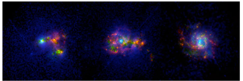 |
Figure 16. Three nearby star-forming galaxies imaged as part of the HST Lyman-α imaging program LARS. Green shows the UV continuum and traces the massive stars, with the ionized nebulae they produce shown in Red (tracing Hα). The Lyman-α photons must also be produced in these nebulae, but the Lyman-α image (shown in Blue) reveals all these galaxies to be morphologically very different in Hα and Lyman-α due to the resonant scattering of the Lyman-α photons. This is at least qualitatively similar to what is found for high-redshift LAEs, in which the Lyman-α emission is in general more extended and diffuse than the UV continuum light (courtesy of Matt Hayes). |
It is easy to become confused by the (extensive) literature on the properties of LAEs. In part this is because different authors adopt a different definition of what is meant by the term LAE. For some, an LAE is any galaxy which displays detectable Lyman-α emission, including objects originally selected as LBGs and then followed up with spectroscopy. All spectroscopically-confirmed LBGs at z > 5 must of course be emitters of Lyman-α radiation, and so in an astrophysical sense they are indeed LAEs. However, in practice most LAE studies are really confined to objects which have been selected on the basis of Lyman-α emission. Furthermore, many of these studies then proceed to deliberately confine attention to those LAEs which could not also have been selected as LBGs from the data in hand. Of course there are often good reasons for doing this. For example, Ono et al. (2010) in their study of the typical UV properties of LAEs at z ≃ 5.7 and z ≃ 6.6 first excised 39 of the 295 LAEs from their sample because they were individually detected at IRAC wavelengths, before proceeding to stack the data for the remaining LAEs to explore their average continuum colours. This makes sense given the objective of this work was to explore the properties of those objects which were not detected with IRAC, but such deliberate focus on the extreme equivalent-width subset of the LAE population does sometimes run the danger of exaggerating the differences between the LBG and LAE populations.
To put it another way, in many respects the properties of LAEs, selected on the basis of large EWrest, are largely as would be anticipated from the extreme Lyman-α equivalent-width tail of the LBG population. I have already argued above that the observational evidence on luminosity functions suggests LAEs are just a subset of LBGs, and that by z ≃ 6 the increased escape of Lyman-α means that the two populations are one and the same. At least some existing HST-based comparisons of LAEs and LBGs support this viewpoint (e.g. Yuma et al. 2010), as do at least some theoretical predictions (e.g. Dayal & Ferrara 2012). It is then simply to be expected that the subset of galaxies selected on the basis of extreme Lyman-α EWrest (and hence also typically faint UV continuum emission) will, on average, have lower stellar masses, younger ages, and lower-metallicities than typical LBGs discoverable by current continuum surveys (e.g. Ono et al. 2012).
At present, therefore, there is really no convincing evidence that LAEs are anything other than a subset of LBGs. This is not meant to denigrate the importance of LAE studies; faint narrow-band selection provides access to a special subset of the UV-faint galaxy population over much larger areas/volumes than current deep HST continuum surveys. But the really interesting questions are whether this extreme equivalent-width subset represents an increasingly important fraction of LBGs with decreasing UV continuum luminosity and, conversely, whether some subset of this extreme equivalent-width population cannot be detected in current deep HST continuum imaging. To answer the first question really requires ultra-deep spectroscopic follow-up at z ≃ 6-7 of objects selected as LBGs spanning a wide range of continuum luminosity M1500. To answer the second question, following Cowie et al. (2011), further deep HST WFC3/IR imaging of objects selected as LAEs is desirable to establish what subset (if any) of the LAE population lacks sufficiently compact UV continuum emission to be selected as a faint LBG given the surface brightness biases inherent in the high-resolution deep HST imaging.
4.3.6. Beyond z ≃ 6.5; a decline in Lyman-α?
Both the follow-up spectroscopy of LBGs, and the discovery of LAEs via narrow-band imaging become increasingly more difficult as we approach z ≃ 7, due to the declining sensitivity of silicon-based detectors at λ ≃ 1 µm , the increasing brightness of night sky emission and, of course, the reduced number density of potential targets (as indicated by the evolution of the LBG luminosity function discussed above). Nevertheless, even allowing for these difficulties, there is now growing (albeit still tentative) evidence that Lyman-α emission from galaxies at z ≃ 7 is signicantly less prevalent than at z ≃ 6. Specifically, while spectroscopic follow-up of LBGs with zphot > 6.5 has indeed yielded several Lyman-α emission-line redshifts up to z ≃ 7 (see section 3.1), these same studies all report a lower success rate (≃ 15-25%) than encountered at z ≃ 6 (Pentericci et al. 2011; Schenker et al. 2012; Ono et al. 2012). In addition, such Lyman-α emission as is detected seems typically not very intense, with an especially significant lack of intermediate Lyman-α equivalent widths, EWrest ≃ 20-55 Å. The significance of the inferred reduction in detectable Lyman-α obviously becomes enhanced if judged against extrapolation of the rising trend in Lyman-α emission out to z ≃ 6, as discussed above, and plotted in Fig. 13 (Stark et al. 2011; Hayes et al. 2011; Curtis-Lake et al. 2012).
These results may be viewed as confirming a trend perhaps already hinted at by the reported modest decline in the Lyman-α luminosity function between z ≃ 5.7 and z ≃ 6.6 (as outlined above in section 4.2), and the tentative (albeit controversial) indications of further decline at z ≥ 7. In summary, there is growing evidence of a relatively sudden reduction in the transmission of Lyman-α photons between z ≃ 6 and z ≃ 7. Given that the galaxy population itself appears, on average, to become increasingly better at releasing Lyman-α photons to the observer out to z ≃ 6 (perhaps due to a global decline in average dust content), the most natural and popular interpretation of this decline at z ≃ 7 is a significant and fairly rapid increase in the neutral hydrogen fraction in the IGM.
This has several implications. First, it suggests that further comparison of LAEs and LBGs over the redshift range z ≃ 6 - 7 may well have something interesting to tell us about reionization (at least its final stages; see section 6.2). Second, it implies that spectroscopic redshift determination/confirmation of LBGs at z > 7 is likely to be extremely difficult, and that, for astrophysical reasons, we may be forced to rely on photometric redshifts at least until the advent of genuinely deep near-to-mid infrared spectroscopy with JWST (capable of detecting longer-wavelength emission lines including Hα). Third it suggests that the spectacular success of LAE selection via narrow-band imaging out to z ≃ 6.6 could be hard to replicate at higher redshifts, and hence that the future study of galaxies and their evolution at z ≃ 7-10 may well be driven almost entirely by Lyman-break selection.