1.1. ORBITS

Even a gas-free galaxy is a formidably complex dynamical system: ∼ 10¹¹ stars and inconceivably more WIMPS are strongly coupled by their mutual gravitational field. As in any branch of theoretical physics we make progress by simplifying. The key simplification is that the motion of all these particles would be very similar if calculated in the gravitational field of an imaginary smoothed-out version of the galaxy. That is, we smear the mass of each particle over something like an interstellar distance and compute the gravitational field from this smooth mass distribution. Given the usefulness of this approximate gravitational field, our first task becomes to understand how particles move in smooth gravitational fields of this kind.

1.1.1. Quasiperiodicity and isolating integrals

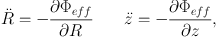
The equations of motion of a particle in a typical gravitational potential Φ are readily integrated numerically. If the potential is axisymmetric, the component of angular momentum about the galaxy's symmetry axis, L_z, is conserved, and we can eliminate the azimuthal angle φ and its time derivative from the equations of motion, leaving us with two coupled ordinary differential equations to integrate:

(1.1)

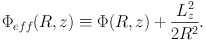
where

(1.2)

Fig. 1.1 shows a couple of typical orbits obtained in this way. They have a nicely regular pattern of paths running to and fro. Given sufficient time such an orbit will carry the particle to any given point inside the bounding envelope, and when it reaches that point the particle will be moving with one of four velocities: = ± v_R and = ± v_z, where v_R and v_z are numbers that depend on the orbit and the location.

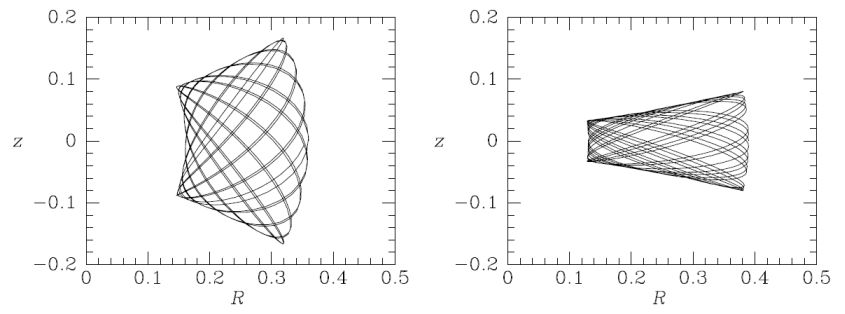Figure 1.1. The motion in the (R, z) plane of a particle that orbits in an axisymmetric gravitational potential. The orbits have the same values of E and Lz but are nevertheless very different because they have different values of the mysterious “third integral”.

If the time series R(t) or z(t) obtained in this way is Fourier transformed, one finds that the spectrum consists of discrete lines, and moreover, any frequency appearing in the spectrum can be expressed as an integer linear combination of two fundamental frequencies Ω_R and Ω_z. That is,

(1.3)

where

(1.4)

with n_R and n_z being (possibly negative) integers. Thus the orbit is characterised by the two fundamental frequencies and countably many amplitudes R_n, z_n and phases ψ_{R n},ψ_{z n}. An orbit with these properties is said to be quasiperiodic.

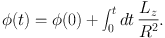
As the particle moves in the (R, z) plane, it rotates about the symmetry axis: its azimuthal coordinate φ can be found by simple quadrature:

(1.5)

The time series of φ will consist of sinusoidal contributions at discrete frequencies superimposed on a secularly increasing value, and the rate of the secular increase defines a third fundamental frequency Ω_φ. Thus three fundamental frequencies will be required to express the frequency of any line in the spectrum of say x(t) as an integer linear combination of fundamental frequencies.

The result of integrating the equations of motion in potentials that are not axisymmetric cannot be displayed as nicely as in Fig. 1.1. But when you Fourier transform the time series x(t) of the coordinates of such orbits, you usually find that the spectra consist of lines that can be expressed as integer linear combinations of three fundamental frequencies. So a large fraction of orbits in galaxy-like potentials are quasiperiodic.

An integral of motion is a function I(x, v) on phase space that returns the same number no matter at what point along an orbit you evaluate it:

(1.6)

We say that I is an isolating integral if the set of phase-space points that satisfy equation (1.6) for some given value on the right side defines a smooth five-dimensional subset of phase space. For example, the energy E(x, v) = 1/2 v² + Φ(x) is an isolating integral.

If an orbit is quasiperiodic, one may show that it admits at least three functionally independent isolating integrals. We can take E to be one of these, and in the case of an axisymmetric potential, L_z = xv_y − yv_x can be taken to be another of them. Only in exceptional potentials do we have an analytic expression for a third isolating integral, but its existence is assured by the quasiperiodic nature of orbits – for a proof see Arnold (1978).

1.1.2. Angles and actions

It often happens that the key to solving a physics problem is to identify the coordinate system that's best suited to that problem. Hamiltonian mechanics allows us to use an extremely wide range of coordinates for phase space with ease – all “canonical coordinates” are intrinsically equal. In the following we shall denote by (x, p) a canonical system made up of coordinate x_i that gives the star's position and its canonically conjugate momentum p_i. In the simplest case x_i is a Cartesian coordinate and p_i = ẋ_i is its rate of change, but in some instances p_i ≠ ẋ_i. Given that three isolating integrals I_i exist, a shrewd question to ask is “is there a canonical coordinate system in which the I_i, or some functions of them, act as momenta?” Since any function J(I₁, I₂, I₃) of the I_i will itself be an integral of motion, we usefully increase our chances of our enquiry having the answer “yes” by opening the enquiry up to functions of our original integrals.

It turns out that only a highly restricted group of integrals are capable of playing the role of momenta. We call such integrals actions and reserve for them the letter J, so J_j(x, p) is the jth action of an orbit.

To understand why only special integrals can act as momenta, we should consider the subset M of points in phase space that satisfy

(1.7)

These equations impose three restrictions on the six phase-space coordinates (x, p). So the set M is a three-dimensional subset of phase space to which the particle is confined for all time. M is a subset of the energy hypersurface H(x, p) = E, where H is the Hamiltonian function and E is the particle's energy. If the orbit is bound, as we shall assume, the energy hypersurface is compact, so M is compact also. In practice M will also be a connected set, and it can then be shown that it is diffeomorphic to a 3-torus (see §§49, 50 of Arnold, 1978, for a proof).

What is a 3-torus? Think of a room with each point on the floor identified with the point on the ceiling that is vertically above it, each point on the left wall identified with the corresponding point on the right wall, and with points on the front and back walls similarly identified. Position within this room (M) is specified by the values of the coordinates θ₁, θ₂ and θ₃ that are canonically conjugate to J₁, J₂ and J₃, whose values specify which room (torus) we are in. They do so in a way that can be understood geometrically.

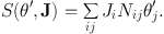
In Hamiltonian mechanics a fundamental role is played by the Poincaré invariant P. This is a number that we assign to any two-surface S in phase space through

(1.8)

so P(S) is the sum of the areas of the projections of S onto all the planes formed by each coordinate x_i and its conjugate momentum p_i. It's called an invariant because you get the same number no matter what canonical coordinates you use. Consequently, given any two-surface S∈ M we can replace (x_i, p_i) by (θ_i, J_i) and write

(1.9)

and this vanishes because every point of S has the same value of J_i. In view of this fact we say M is null. It follows from the nullness of M that the value of any line integral ∫ dx · p through M between two given endpoints is the same for any path between those points that can be continuously distorted into some standard path without leaving M. To see why, take the difference between the integrals along two different paths Γ₁ and Γ₂ between a given pair of points. This difference of integrals is identical with the line integral along the closed path Γ₁ − Γ₂ in which we go out on Γ₁ and back on Γ₂. By Green's theorem this closed line integral is equal to the Poincaré invariant of the 2-surface that Γ₂ sweeps out as it is deformed into Γ₁. But this Poincaré invariant vanishes, so the original line integrals were equal. Consider now the line integral ∫ dx · p along the path from the front wall to the corresponding point on the back wall. We choose to evaluate this integral using the (θ, J) coordinates, and to take the path on which θ₂=θ₃=constant. Then we have

(1.10)

so J₁ is equal to ∫ dx · p divided by the amount by which θ₁ increments as we cross the room. We choose to scale the actions so θ_i increments by 2π on crossing the room, so

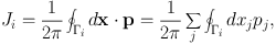(1.11)

where Γ_i is any path that takes us once across the room.

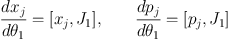
If we want to find the values of the ordinary phase-space coordinates (x, p) at the point θ we need to do the following: (i) Choose a point (x₀, p₀) in the room and declare it to be θ = 0. Now integrate from the initial conditions x = x₀, p = p₀ when θ₁ = 0 the coupled o.d.e.s

(1.12)

where [..] denotes a Poisson bracket, to discover the (x, p) coordinates of the points θ = (θ₁, 0, 0). (ii) Starting from any of these points we can integrate the o.d.e.s

(1.13)

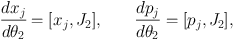
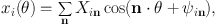
to discover the (x, p) coordinates of the points θ = (θ₁, θ₂, 0). (iii) Starting from any of the last-mentioned points we can integrate the third set of o.d.e.s to find the (x, p) coordinates of a general point θ. The key property of actions is that if we integrate say the first set of o.d.e.s from a point θ_a on one wall to the point θ_b at which the trajectory hits the opposite wall, we find that θ_b = θ_a + (2π, 0, 0) (Fig. 1.2 left). That is the trajectories generated by actions carry you from a point on one wall to the point on the opposite wall that we have identified with our starting point. If we form some other integrals I_i(J) by adopting three non-trivial functions of the actions, the trajectories generated by the I_i will not carry us from a point on a wall to the point on the opposite wall that has been identified with it (Fig. 1.2 right). Consequently, the variables that are canonically conjugate to the I_i cannot form a global coordinate system (although they can be used as coordinates locally).

Figure 1.2. Trajectories generated by an action (left) and by some other integral (right). In the left panel each horizontal curve joins points on the left and right boundaries that have been identified, whereas in the right panel the leftmost and rightmost points of these curves are at logically distinct points. Consequently, in the right panel the periodic continuation of each horizontal curve would not overlie the portion plotted. The vertical curves exhibit the same phenomenon. Consequently these curves define a global coordinate system only in the left panel.

In remembrance of the fact that θ_a and θ_b = θ_a + (2π, 0, 0) correspond to the same point in phase space, the canonically conjugate coordinates of actions are called angle variables. To see what flexibility we have in the choice of actions and angles, we observe that if we have new variables θ′ that are related to our original angle variables by linear equations

(1.14)

where n is a matrix with integer entries, then if any of the θ′_i is incremented by 2π, all the θ_j will change by 2mπ, so we will return to the same place in phase space. Hence the θ′ provide a global coordinate system for a torus as effectively as the θ. To discover what actions correspond to the θ′, we write down the generating function of the canonical transformation (θ, J) ↔ (θ′, J′)

(1.15)

It is straightforward to check that S generates equation (1.14) and we have also

(1.16)

Thus the new actions are integer linear combinations of the old actions.

Any function on phase space can be expressed as a function of the angles and actions (θ, J). In particular the Hamiltonian can be expressed in this form. But while the angle variables vary as a particle orbits, its energy does not. So the Hamiltonian cannot depend on θ. Hence the Hamiltonian is a function H(J) of the actions only. This fact makes the equations of motion of the angle variables trivial:

(1.17)

Since H depends on J only, so must its partial derivatives Ω_i. Since J is constant along the orbit, Ω_i is too, so we can immediately integrate equation (1.17):

(1.18)

Thus the particle moves through its room at constant speed along straight lines whose slope is given by Ω = ∂ H / ∂ J.

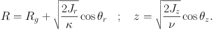
Usually the frequencies are incommensurable and then the line will eventually come arbitrarily close to every point in the room (Fig. 1.3 left).

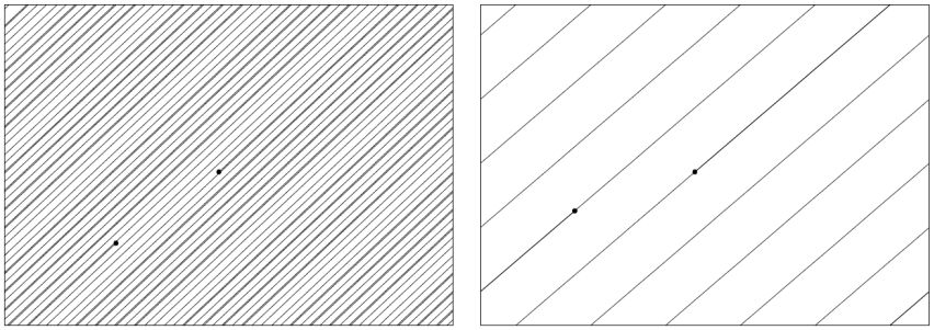Figure 1.3. A particle moves through its room (torus) on a straight line that repeatedly hits a wall and reappears at the corresponding point on the opposite wall. If the components of the slope vector are rationally related, the line eventually closes on itself (right). In general it does not close and comes arbitrarily close to every point in the room (left). Black dots mark the start and end of the plotted portion of the trajectory.

Since the ordinary phase-space coordinates are periodic functions of the angle variables with period 2π they can be expanded in Fourier series

(1.19)

where the sum is over vectors with integer components and the X_in and ψ_in are constant amplitudes and phases. When we substitute into this expression our solution (1.18) of the equations of motion, we obtain

(1.20)

Equation (1.3) from which we started is an instance of this equation. Thus we have come full circle from the empirical fact that numerically integrated orbits are quasiperiodic to the fact that such spectra are a necessary consequence of these orbits having three isolating integrals.

In the generic case of incommensurable frequencies, we have a useful result, the time-averages theorem: when the frequencies are incommensurable, the fraction of its time a particle spends in a subset V of the torus is ∫_V d³ θ / (2π)³. From this the strong Jeans theorem follows: in a steady-state galaxy, the density of stars is uniform within incommensurable tori, so the density of stars in phase space is a function f(J) of the actions only. We call f the distribution function, often abbreviated DF.

It is useful to think of orbits as points in the three-dimensional space, action space, that has the three actions as is Cartesian coordinates. The strong Jeans theorem tells us that galactic equilibria are simply distributions of stars in this easily imagined space.

1.1.3. Epicycle approximation

It's instructive to examine a very useful model at this point. A star in an axisymmetric potential moves in the effective potential (1.2). It is physically obvious that the minimum of Φ_eff occurs at (R_g, 0), where the guiding-centre radius R_g is the radius of the circular orbit with the given angular momentum L_z. Since this is the potential's minimum, a Taylor expansion of Φ_eff around it will contain no linear terms and be of the form

(1.21)

Stars on sufficiently circular orbits will be confined to the region in which we need retain only the first three terms in this series. Consequently, their radial and vertical motions will be harmonic. The frequencies of these oscillations are Ω_r = κ, the epicycle frequency and Ω_z = ν, the vertical epicycle frequency. The solution to the equations of motion is

(1.22)

where X, ψ_r, Z and ψ_z are all constants. Clearly we can set

(1.23)

Then calculating p_R = and evaluating ∮d R p_R we can show that X = √2J_r / κ, and similarly that Z = √2J_z / ν, so in the epicycle approximation the connection between ordinary coordinates and angle-action variables is

(1.24)