1.2. RESONANCES

The fundamental frequencies Ω are generally non-trivial functions of the actions, so for certain tori a resonance condition N · Ω = 0 will apply. When we multiply the resonance condition by t and use equation (1.18), we obtain

(1.25)

This equation inspires us to make a canonical transformation to new angles and actions (θ′, J′) such that N · θ becomes one of the new angles, say θ′₁. It does not much matter what we adopt for θ′₂ and θ′₃; θ′₂ = θ₂ and θ′₃ = θ₃ works fine. Then our generating function becomes

(1.26)

so the new angles are

(1.27)

Since θ′₁ does not evolve in time, the star explores only a two-dimensional set of its three-dimensional torus. While a star on a resonant torus does not come arbitrarily close to every point on its torus, the bigger the numbers N_j are, the more effectively it samples its torus, and the less likely it is that the resonance condition will be dynamically important.

1.2.1. Perturbation theory

The importance of resonances only emerges when we consider the effects of adding a small perturbing Hamiltonian h(θ, J) to the Hamiltonian H₀(J) for which we have found angle-action variables (θ, J). We use these coordinates to study the motion of a particle in the full Hamiltonian H = H₀ + h. Hamilton's equations read

(1.28)

where Ω₀ = ∂ H₀ / ∂J. The perturbing Hamiltonian, like any function on phase space, is a periodic function of the angles, so we can Fourier expand it:

(1.29)

With this expansion, the equation of motion of J is

(1.30)

So long as n · Ω ≠ 0, the time-averaged value of J vanishes and we expect J simply to oscillate slightly around its unperturbed value. But if a resonance condition is nearly satisfied, N · Ω ≃ 0, the argument of one or more of the sines will change very slowly, and the cumulative change in J can be significant even for very small h_n. Thus resonances permit small forces to act in the same sense for long times, and hence cause qualitative changes in behaviour. This is one of the fundamental principles of physics.

Mathematically, we use the new angle variables θ′ defined by equation (1.27) and their conjugate actions

(1.31)

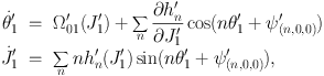
Next we express h as a Fourier series in the new angle variables and discard all terms that involve θ′₂ or θ′₃ on the grounds that they oscillate too rapidly to have a significant impact on the dynamics. Since our approximated Hamiltonian depends on neither θ′₂ nor θ′₃, the conjugate actions J′₂ and J′₃ will be constants of motion. The only non-trivial equations of motion are now

(1.32)

where

(1.33)

and we have suppressed the dependence of Ω₀₁ and h′_n on J′₂ and J′₃ because the latter are mere constants. We have reduced the particle's motion in six-dimensional phase space to motion in the (θ′₁, J′₁) plane.

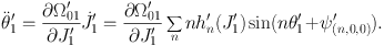
We differentiate with respect to time the first of equations (1.32)

(1.34)

We can neglect the sum in this equation because each of its terms is the product of a derivative of h′_n, which is small, and either J′₁, which is of the same order, or θ′₁, which is also small because Ω′₀₁ vanishes at the resonance. Therefore we can dramatically simplify the θ′₁ equation of motion to

(1.35)

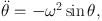
If we approximate ∂ Ω′₀₁ / ∂ J′₁ and h′_n by their values on resonance, and retain only the term for n = 1 in the sum, we are left with the equation of motion of a pendulum

(1.36)

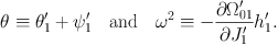
where

(1.37)

A pendulum can move in two ways: at low energy its motion is oscillatory at an angular frequency that falls from ω at the lowest energies to zero at the critical energy above which the pendulum circulates. Consequently, equation (1.35) predicts that close to the resonance (“low energy”) θ′₁ will oscillate. This is the regime of resonant trapping in which the particle librates around the underlying resonant orbit. At some critical distance from the resonance (“high energy”) θ′₁ will start to circulate. Near the threshold energy, the rate at which θ′₁ advances in time will be highly non-uniform, just as a pendulum that has only just enough energy to get over top dead centre slows markedly as it does so. As we move further and further from the resonance, the rate of advance of θ′₁ becomes more and more uniform, and we gradually recover the unperturbed motion, in which the rate of advance of θ′₁ is strictly uniform.

We can obtain a useful pictorial representation of this behaviour by deriving the energy invariant of equation (1.36). We multiply both sides by θ to obtain an equation which states that

(1.38)

is constant. Consequently, the particle moves in the (θ,θ) plane along curves of constant E. These curves are shown in Fig. 1.4. The round contours near the centre of the figure show the motion of a particle that has been trapped by the resonance, while the contours at the top and bottom of the figure that run from θ = −π to θ = π show the motion of a particle that continues to circulate.

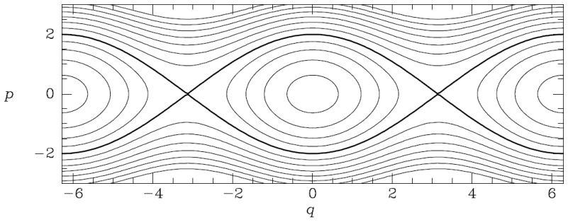Figure 1.4. The phase plane of a pendulum. Curves of constant energy E (eq. 38) are plotted. The particle moves on these, from left to right in the upper half of the figure and from right to left in the lower half.

To appreciate the significance of resonances for galactic dynamics we must introduce the concept of a surface of section. This is a phase plane such as the (R, p_R) plane for motion in an axisymmetric potential. Each time the particle passes through the plane z = 0 moving upward (p_z > 0) we mark the surface of section with a dot at the current values of R and p_R. If the orbit is quasiperiodic, the dots eventually trace out a curve. This curve is the intersection of the orbit's torus with the (R, p_R) plane, and in fact the area inside it, ∫ d R d p_R is 2π times the orbit's radial action J_r. Fig. 1.5 shows surfaces of section for motion in two flattened axisymmetric potentials. In a given panel each curve is for a different orbit with the same energy and value of L_z. Most of the curves move around a central point. The point itself is made by the shell orbit, which is two-dimensional and has J_r = 0; in real space this orbit is a thin cylindrical shell that has a larger diameter at z = 0 than at its top or bottom edges. Each curve around this point in Fig. 1.5 is generated by a three-dimensional orbit that forms an annulus of finite thickness. Fig. 1.1 shows cross sections through two such annuli. In Fig. 1.5, the longer an orbit's curve is, the thicker the annulus and the smaller its vertical extent. The outermost curve in Fig. 1.5 is generated by the orbit J_z = 0, which is confined to the plane z = 0. So in Fig.1 the orbit in the left panel generates a larger curve in the left panel of Fig. 1.5 than does the orbit of the right panel of Fig. 1.1.

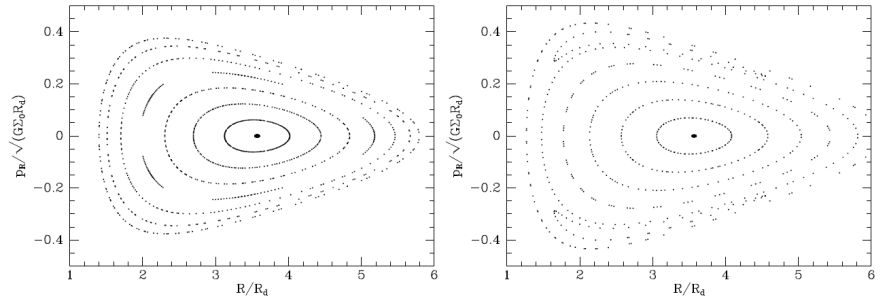Figure 1.5. Surfaces of section for motion in flattened isochrone potentials: the left panel is for the case of a mass distribution that has axis ratio q = 0.7, while the right panel is for q = 0.4. In the right panel we see resonant islands generated by the 1:1 resonance between the radial and vertical oscillations. No such island is evident in the left panel.

The right panel in Fig. 1.5 is for motion in the potential of a flatter galaxy than the left panel, and in this panel not all curves loop around the central point. Two resonant islands have appeared, formed by orbits that have been trapped by the resonance Ω_r = Ω_z.

At this point one should be asking “so what's the perturbation in this case?” It isn't evident that there is one; all we did was integrate orbits in a perfectly well defined potential. However, we can imagine that our Hamiltonian is the sum of a Hamiltonian H₀ that would generate a surface of section in which all curves simply looped around the central point, and a smaller Hamiltonian h = H − H₀, and to ascribe to h the trapping of orbits by the 1:1 resonance. Kaasalainen & Binney (1994) describe an algorithm that can be used to generate H₀ and h.

The resonance just discussed is rather a tame one that probably does not play a big role in galactic dynamics (but see § 1.2.3). Resonances certainly play a big role in the dynamics of bars. The dynamics of a bar is strongly affected by the bar's pattern speed, Ω_p, the angular velocity at which the figure of the bar rotates. The bars we see at the centres of more than half spiral galaxies, including our own, are rapidly rotating in the sense that in the rotating frame of the bar the dynamics of most stars depends strongly on the Coriolis force 2 Ω_p × p. In cosmological simulations of the clustering of dark matter, most dark halos are barred and their pattern speeds are so small that the Coriolis force is unimportant for a significant fraction of their constituent particles. The gravitational potentials of galaxies are approximately isothermal, so let's investigate motion in the potential

(1.39)

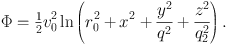
Here r₀ is a core radius, within which the potential tends towards that of a harmonic oscillator, and v₀ would be the circular speed at x≫ r₀ in the (x, y) plane if the axis ratio q were unity. We shall assume that q = 0.8, so the potential is slightly elongated along the x axis and for now restrict ourselves to motion in the (x, y) plane so we can use the device of a surface of section.

Fig. 1.6 shows (x, p_x) surfaces of section for two values of r₀. In the case r₀ = 0.1 on the left we can identify the curves of two types of orbit: the two bulls-eyes comprise the curves of loop orbits such as that depicted in the top left panel of Fig. 1.7. These orbits have a well-defined sense of rotation about the z axis. The curves that surround both bulls-eyes are generated by box orbits such as that depicted in the bottom left panel of Fig. 1.7. Box orbits extend to the potential's centre and do not involve rotation. In the surface of section on the right of Fig. 1.6 we see several resonant islands in the domain of the box orbits. These islands are made up of orbits trapped by the resonances Ω_y = 2Ω_x (outermost island) and 2Ω_y = 3Ω_x (further in). The right panels of Fig. 1.7 show the appearance of a couple of these orbits in real space. As this experiment suggests, the more cuspy a triaxial mass distribution is, the larger is the fraction of phase that is occupied by resonant box orbits, or boxlets as they have been called (Merritt & Valluri, 1999). Why resonant trapping becomes more important as the matter distribution becomes more cuspy is not clear. A fact that is probably relevant is that boxlets generally avoid the galactic centre, while boxes do not. Given that massive black holes reside in galaxy centres, the tendency of boxlets to avoid the centre clearly has important astrophysical consequences by keeping stars safe from being eaten by the monster there.

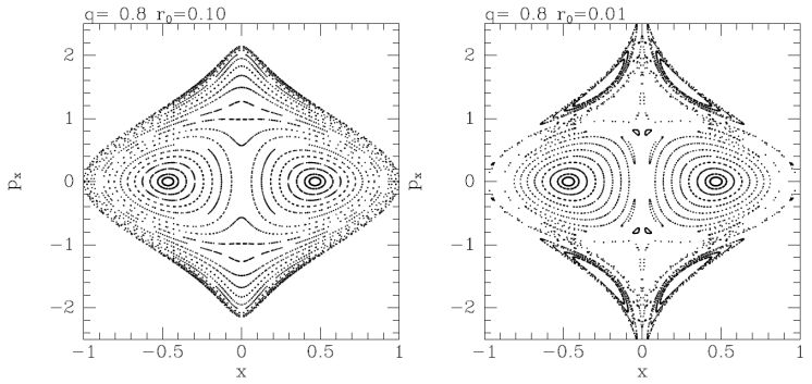Figure 1.6. Surfaces of section for the potential (1.39) with axis ratio q = 0.8. Left: for r0 = 0.1; right: for r0 = 0.01.

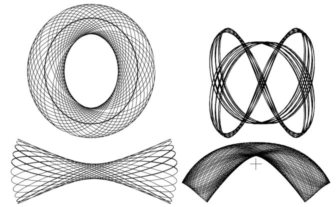Figure 1.7. A loop and a box orbit (left); two boxlets (right). The cross in the lower right panel marks the potential's centre.

1.2.2. Frequency analysis

We have seen how surfaces of section give valuable insight into the structure of phase space. Unfortunately, it is impracticable to construct a surface of section unless the motion is in two dimensions – or effectively so in the case of an axisymmetric potential. Frequency analysis provides a useful way of determining which resonances play an important role when the potential is triaxial and the motion of particles is inherently three-dimensional. The technique consists of numerically integrating orbits and then Fourier transforming the time dependence of suitable coordinates. From the resulting spectra one identifies the fundamental frequencies, and determines two frequency ratios, such a Ω_z / Ω_x and Ω_z / Ω_y. Each orbit then generates a point in a frequency-ratio diagram such as that of Fig. 1.8. In this diagram the points of non-resonant orbits fall along a curvilinear grid, which reflects the systematic way in which the initial conditions explored phase space. The points of resonant orbits lie along straight lines. In the vicinity of these lines there is a deficit of points, because orbits in the underlying integrable potential that would have the nearly commensurable frequencies that correspond to these locations have been resonantly trapped so their principal frequencies exactly satisfy a resonance condition. Actually these orbits still have three independent fundamental frequencies, but one of these frequencies is the frequency of libration around the trapping orbit, and this frequency has to be dug out of the coordinates' spectra and is missed by the simple algorithm from used to identify the frequencies from which the frequency ratios were calculated.

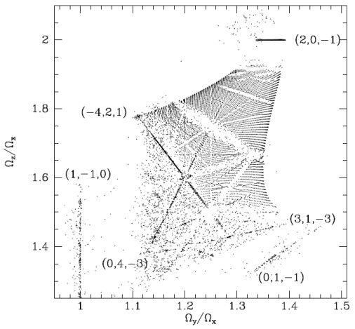Figure 1.8. Frequency-ratio diagram for the potential (1.39) with q = 0.9 and q2 = 0.7.

1.2.3. Adiabatic deformation

The Milky Way's disc has accumulated rather gradually over most of the Hubble time. As it grew, the Galaxy's potential must have deformed from being the nearly spherical potential of the dark halo, to a potential that is significantly pinched towards the plane (Fig. 1.9). Individual orbits will have distorted in response to the distortion of the potential, but so long as they remained non-resonant, their actions will have been invariant: actions are adiabtatic invariants. This fact greatly facilitates the process of determining the response of a stellar system to adiabatic distortion of its potential because all we have to do is to move each star from its orbit in the original potential to the orbit with the same actions in the distorted potential. In particular, the structure of the distorted system depends only on the initial and final configurations, and not on which configurations it passed through in between.

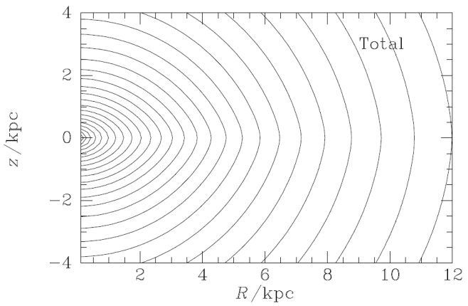Figure 1.9. A model Galaxy potential. The cuspiness of the equipotential contours clearly show the extent to which the potential has been flattened by the mass of the disc.

Fig. 1.5 shows surfaces of section for motion in a potential before and after the resonance condition Ω_r = Ω_z is first satisfied: the islands visible in the right panel are made up of orbits trapped by this resonance. Note that the areas of the curves in the left panel are 2π J_r, so they do not change as the potential flattens.

The resonance condition is first satisfied by the orbit that is confined to the equatorial plane; in both panels of Fig. 1.5 the curve of this orbit lies on the outside. Hence the resonant islands first appeared just inside this curve. As the potential flattened more, Ω_r / Ω_z dropped significantly below unity for the planar orbit, so the resonance condition was satisfied by orbits with non-zero J_z and the islands moved inwards. Orbits whose curves lay in the path of a moving island did one of two things: (a) they were trapped into the island, or (b) they abruptly increased their radial actions so that their curves went round the far side of the island. Which of these two outcomes happened in an individual case depended on the precise orbital phase of the star when the potential achieved a particular flattening, but it is most useful to average over phases and to consider the outcomes to occur with probabilities P_a or P_b. The magnitudes of P_a and P_b depend of the relative speed with which the island increased its area and moved: if it simply grew, P_a = 1, and if it moved without growing P_b = 1. These results follow from Liouville's theorem that phase-space density cannot increase.

Let's imagine that after a period of stationary growth, the island moved inwards without growing, and then became stationary while it shrank. In this case it would have swept up stars with large J_r and small J_z and released these stars into orbits with smaller J_r and larger J_z. In other words, it will have turned radial motion into vertical motion. Sridhar & Touma (1996) have called this process “levitation”. Conversely, the moving island will have reduced the vertical motions and increased the radial motions of any stars it found in its path through action space. Thus resonances stirr the contents of phase space. Levitation is a lovely idea but it's not clear that it is of practical importance. We shall see below that in a disc analogous scattering by resonances is very important.

1.2.4. From order to chaos

If we set z = 0 and express the triaxial potential (1.39) in cylindrical coordinates, it becomes

(1.40)

Consider now the related potential (Binney, 1982)

(1.41)

Fig. 1.10 shows surfaces of section for motion in this potential when r₀ = 0.1, q = 0.9 and R_e = 6 (left) and R_e = 4 (right). Comparing the left panel of this figure with the left panel of Fig. 1.6 we see that the extra term in the logarithm has greatly increased the number of resonant islands, and in the right panel we see that it can introduce a qualitatively new feature: many points seem now to be scattered at random rather than confined to curves. Confinement to curves is an indication that the orbits admit an isolating integral in addition to energy, and are in consequence quasiperiodic. Conversely, when the points are not confined to curves, the orbits lack an additional integral and are not quasiperiodic. We say these orbits are irregular or chaotic.

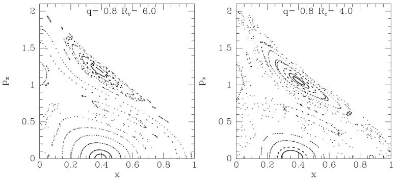Figure 1.10. Surfaces of section for the potential (1.41) with q = 0.8 and r0 = 0.1. The left panel is for Re = 6 and the right panel is for Re = 4.

The increase in the number of resonant islands is probably the cause of the emergence of chaos. In the surface of section, islands form chains, with the curves of some non-trapped orbits running on one side of the chain, and those of others running on the other side of the chain – Fig. 1.4 may help the reader to picture this situation. The curves of the most nearly trapped orbits on each side come very close where the islands touch. The tiniest perturbation can cause a star on one of these orbits to swap from one side of the chain to the other. If a star makes such changes, its orbit ceases to be quasiperiodic.

If there are several chains of islands in the surface of section, and the islands of two chains almost touch, a star can make two such swaps, moving from, say, inside chain 1 to outside chain 3. In this way a star can move stochastically through a significant region of phase space. This is probably what happens in Fig. 1.10.