


Parametric profiles have been extremely successful in modeling cluster mass distributions derived from observed lensing data. A key advantage of parametric models is their flexibility, as they can be used to probe the granularity of the mass distribution on a range of spatial scales. For the case of clusters, this enables combining strong and weak lensing data that derive from different regions of clusters in an optimal fashion. Below we outline the lensing properties of three most commonly used mass distributions: the circular Singular Isothermal Sphere [SIS]; the truncated isothermal mass distribution with a core that can be easily extended to the elliptical case [PIEMD] and the Navarro-Frenk-White [NFW] profile. While most mass distributions can be generalized to the elliptical case, there are not always simple and convenient analytic expressions available for lensing quantities as readily as for the PIEMD model. The availability of analytic expressions for the surface mass density, shear and magnification have made the PIEMD a popular choice for modeling lensing clusters.
A.1. The Singular Isothermal Sphere
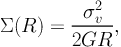
The primary motivation for the circular singular isothermal sphere (SIS) profile derives from the good fit that it provides to the observed approximately flat rotation curves of disk galaxies. Flat rotation curves can be reproduced with a model density profile that scales as ρ ∝ r−2. Such a profile with a constant velocity dispersion as a function of radius appears to provide a good fit to cluster scale halo lenses as well (see e.g. Binney & Tremaine 1987 for more details). The projected surface mass density of the SIS is given by:
 |
(59) |
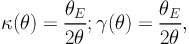
where R is the distance from the center of the lens in the projected lens plane and where σv is the one-dimensional velocity dispersion of ‘particles' that trace the gravitational potential of the mass distribution. The dimensionless surface mass density or convergence is defined in the usual way in units of the critical surface density. For the case of the SIS we have:
 |
(60) |
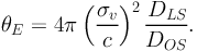
where θ = R / DOL is the angular distance from lens center in the sky plane and where θE is the Einstein deflection angle, defined as
 |
(61) |
Lensing properties of SIS lens model in a nutshell:
A.2. Truncated Isothermal Distribution with a Core
Although the SIS is the simplest mass distribution, it is unphysical as it has an infinite central density, an infinite total mass, and therefore cannot adequately match true mass distributions. More complex mass distributions have therefore been developed to provide more realistic fits to observed clusters. The Truncated Isothermal Distribution with a Core, which has finite mass and a finite central density is quite popular as a lensing model, and one that we have used extensively and successfully in modeling cluster lenses.
The density distribution for this model is given by:
 |
(62) |
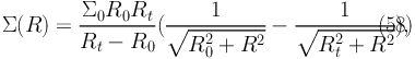
with a model core-radius R0 and a truncation radius Rt ≫ R0.
The useful feature of this model, is the ability to reproduce a large range of mass distributions from cluster scales to galaxy-scales by varying only the ratio η, that is defined as η = Rt / R0. There also exists a simple relation between the truncation radius of the mass distribution and the effective radius Re of the light distribution for the case of elliptical galaxies:
 |
(63) |
Furthermore, this simple circular model can be easily generalized to the elliptical case (Kassiola & Kovner 1993; Kneib et al. 1996) by re-defining the radial coordinate R as follows:
 |
(64) |
Interestingly, all the lensing quantities can be expressed analytically (although using complex numbers) and the expressions for the same were first derived in Kassiola & Kovner (1993).
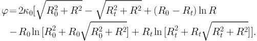
The mass enclosed within radius R for the model is given by:
 |
(65) |
and the total mass, which is finite, is:
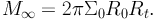 |
(66) |
Calculating κ, γ and g, we have,
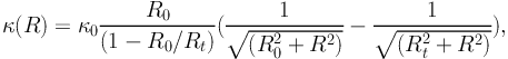 |
(67) |
with:
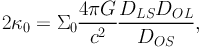 |
(68) |
where DLS, DOS and DOL are respectively the lens-source, observer-source and observer-lens angular diameter distances.
To obtain the reduced shear g(R), given the magnification κ(R), we solve Laplace's equation for the projected potential ϕ, and evaluate the components of the amplification matrix following which we can proceed to solve directly for γ(R), and then g(R).
 |
(69) |
We can then derive the shear γ(R);
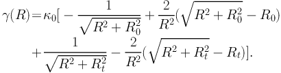 |
(70) |
Scaling this relation by Rt gives for R0 < R < Rt:
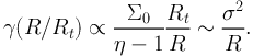 |
(71) |
where σ is the velocity dispersion (note this is similar to the SIS case).
At larger radius, for R0 < Rt < R:
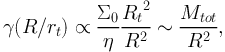 |
(72) |
where Mtot is the total mass. In the limit that R ≫ Rt, we have,
 |
(73) |
Lensing properties of the truncated isothermal distribution with a core in a nutshell:
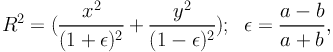
A.3. The Navarro-Frenk-White Model
Although the truncated isothermal distribution with a core is very popular, it has never been fitted to the results of numerical simulations, in contrast to the universal “NFW” density profile (Navarro, Frenk & White 1997). In simulations of structure formation and evolution in the Universe, the NFW profile was found to be a good fit for a wide range of dark matter halo masses from 109 −1015 M⊙. The spherical NFW density profile has the following form:
 |
(74) |
where ρs and rs are free parameters. It is often convenient to characterize the profile with the concentration parameter, cvir = rvir / rs where rvir is the virial radius. By integrating the profile out to rvir and using mvir = 200ρc(z) 4π rvir3/3, where mvir is defined to be the virial mass and ρc is the critical density of the universe, the concentration parameter can be related to ρs.
We now proceed to calculate the lensing properties of the NFW profile (more details can be found in Wright & Brainerd 2000). In the thin lens approximation, z is defined as the optical axis and Φ(R, z) the three-dimensional Newtonian gravitational potential – where r = √R2 + z2. The reduced two-dimensional lens potential in the plane of the sky is given by:
 |
(75) |
where
 =
(θ1, θ2) is the angular position
in the image plane.
=
(θ1, θ2) is the angular position
in the image plane.
For convenience we introduce the dimensionless radial coordinates
 = (x1, x2) =
 / rs =
/ θs where θs = rs
/ DOL. In the case of an axially symmetric lens, the
relations become simpler, as the position vector can be replaced by its
norm. The surface mass density then becomes
/ rs =
/ θs where θs = rs
/ DOL. In the case of an axially symmetric lens, the
relations become simpler, as the position vector can be replaced by its
norm. The surface mass density then becomes
 |
(76) |
with
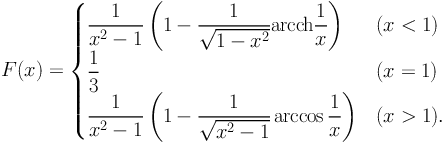 |
and the mean surface density inside the dimensionless radius x is
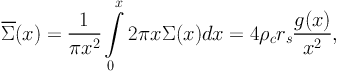 |
(77) |
with
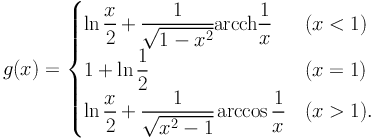 |
The lensing functions
 , κ
and γ also have simple expressions :
, κ
and γ also have simple expressions :
 |
(78) |
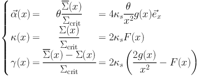
with κs = ρc
rsΣcrit−1. Noting
 α(x) = (∂x1 α,
∂x2 α) and φ =
arctan(x2 / x1),
we obtain some useful relations for the following that hold for any
circular mass distribution
(Golse & Kneib 2002):
α(x) = (∂x1 α,
∂x2 α) and φ =
arctan(x2 / x1),
we obtain some useful relations for the following that hold for any
circular mass distribution
(Golse & Kneib 2002):
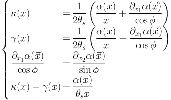 |
(79) |
By integrating the deflection angle we obtain the lens potential ϕ(x):
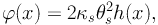 |
(80) |
where
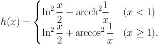 |
(81) |
The velocity dispersion σ(r) of this potential, computed with the Jeans equation for an isotropic velocity distribution, gives an unrealistic central velocity dispersion σ(0) = 0. In order to compare the pseudo-elliptical NFW potential with other potentials, we define a scaling parameter vc (characteristic velocity) in terms of the parameters of the NFW profile as follows:
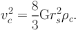 |
(82) |
Using the value of the critical density for closure of the Universe ρcrit = 3H02 / 8π G, we find
 |
Lensing properties of the NFW model in a nutshell:
A.4. Flexion for the Singular Isothermal Sphere
For a Schwarzschild lens: by definition the first flexion is zero everywhere except at the origin. This is of course due to the fact that the gradient of the convergence is zero. A Schwarzchild lens does produce "arciness" in the image. This effect is captured by construction by the second flexion. Expressions for the first and second flexion generated by the mass distribution of a singular isothermal sphere have been provided by Bacon et al. (2005). We reproduce their notation and consistent with our description in section 2.4. The flexion produced by the SIS at angle θ, measured from the centre of the lens is given by:
 |
(83) |
where φ is the position angle with respect to the lens.
The first flexion  for the
SIS profile can be written as a vector and its direction points radially
inward.
for the
SIS profile can be written as a vector and its direction points radially
inward.
The second flexion  , as per
the notation of
Bacon et al. (2005)
is given by:
, as per
the notation of
Bacon et al. (2005)
is given by:
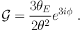 |
(84) |
has a larger peak value
than the first flexion for the
SIS, although both and
fall off with the same power
law index away from the lens. For the explicit derivation of the flexion
for more complicated density profiles, namely the softened isothermal sphere
and the cosmologically motivated Navarro-Frenk-White profile, see
Figure 47 for a comparison as well as
Bacon et al. (2006).
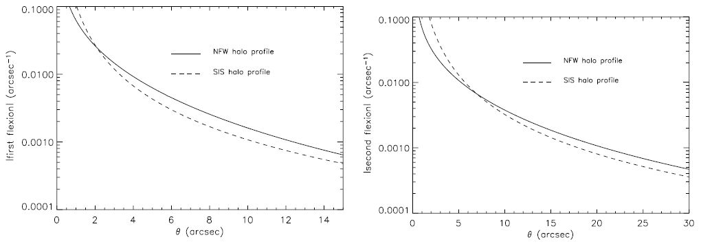 |
Figure 47. Top: Comparison of the magnitude of first flexion due to a NFW and a SIS halo of M200 = 1 × 10¹² h−1 M⊙ at redshift zlens = 0.35. Middle: A similar Flexion1 comparison but this time the SIS halo has M200 = 1.8 × 10¹² h−1 M⊙. Bottom: The magnitude of Flexion2 for a NFW and a SIS halo of M200 = 1 × 10¹²h−1 M⊙, where the doubling in scale of the angular separation axis highlights the larger range and amplitude of the second flexion. |