


Clusters of galaxies are the largest and most massive bound structures in the Universe. Due to their large mass, galaxy clusters (as do galaxies) locally deform space-time (see Figure 3). Therefore, the wave front of light emitted by a distant source traversing a foreground galaxy cluster will be distorted. This distortion occurs regardless of the wavelength of light as the effect is purely geometric. Moreover, for the most massive clusters the mass density in the inner regions is high enough to break the wave front coming from a distant source into several pieces, thereby occasionally producing multiple-images of the same single background source. Background galaxies multiply imaged in this fashion tend to form the observed extraordinary gravitational giant arcs that characterize the so-called strong lensing domain. Strongly lensed distant galaxies will thus appear distorted and highly magnified. They are often referred to as arclets due to their noticeably elongated shape and preferential tangential alignment around the cluster center. Note however that their observed distorted shape is a combination of their intrinsic shape and the distortion induced by the lensing effect of the cluster.
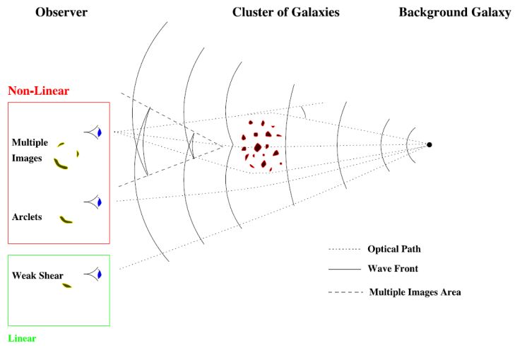 |
Figure 3. Gravitational lensing in clusters: A simple schematic of how lensed images are produced delineating the various regimes: strong, intermediate and weak lensing (see text for a detailed description). |
When the alignment between the observer, a cluster and distant background galaxies is less perfect, then the distortion induced by the cluster will be less important and cannot be recognized clearly. Statistical methods are required to detect this change in shape of background galaxies seen in the weak regime. In the weak lensing regime, the observed shapes of background galaxies in the field of the cluster are typically dominated by their intrinsic ellipticities or even worse by the distortion of the imaging camera optics and the imaging point spread function (PSF) which is a function of position on the detector and may also vary with time. Thus, only a careful statistical analysis correcting the observed images for the various non-lensing induced distortion effects can reveal the true weak lensing signal. The shape changes induced in the outskirts of clusters in the weak regime are at the few percent level, while the strong lensing distortions are often larger, and are typically at the 10% - 20% level.
2.2. Gravitational Lens Equation
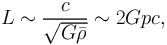
Before proceeding to the elegant mathematics of lensing, we first recap the assumptions needed to derive the basic lens equation. First, it is assumed that the "Cosmological Principle" (i.e. the Universe is homogeneous and isotropic) holds on large scales. The scales under consideration here are the ones relevant to the long-range gravitational force:
 |
(1) |
where c is the speed of light, G is the gravitational
constant and
 is
the mean density of the Universe. The large scale
distribution of galaxies as determined by surveys like the 2 degree Field
survey (2dF), the Sloan Digital Sky Survey (SDSS) and the Cosmic
Microwave Background (CMB) as revealed by the Cosmic Background Explorer
(COBE), and the Wilkinson Anisotropy Probe (WMAP) satellites are in good
agreement with the cosmological principle. The assumption of homogeneity
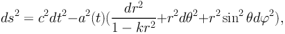
and isotropy imposes strong symmetries on the metric that describes the
Universe and allows solutions that correspond to both expansion and
contraction. Symmetries restrict the metric that describes space-time to
the following form:
is
the mean density of the Universe. The large scale
distribution of galaxies as determined by surveys like the 2 degree Field
survey (2dF), the Sloan Digital Sky Survey (SDSS) and the Cosmic
Microwave Background (CMB) as revealed by the Cosmic Background Explorer
(COBE), and the Wilkinson Anisotropy Probe (WMAP) satellites are in good
agreement with the cosmological principle. The assumption of homogeneity
and isotropy imposes strong symmetries on the metric that describes the
Universe and allows solutions that correspond to both expansion and
contraction. Symmetries restrict the metric that describes space-time to
the following form:
 |
(2) |
where a(t) is the scale factor, and k defines the curvature of the Universe.
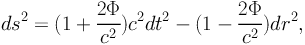
This metric will be locally perturbed by the presence of any dense mass concentration, such as individual stars, black holes, galaxies or clusters of galaxies. The Schwarzschild solution (e.g. Weinberg 1992) gives the form of the metric near a point mass, and is easy to generalize for a continuous mass distribution in the stationary weak field limit corresponding to Φ << c2:
 |
(3) |
where Φ is the 3D gravitational potential of the mass distribution under consideration.
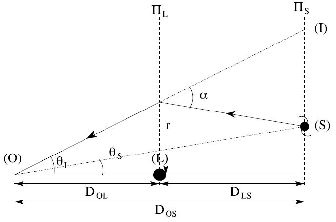 |
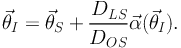
Figure 4. A single deflector lensing configuration showing the relevant angles and distances that appear in the lens equation. |
If we consider a simple configuration of a single thin deflecting lens
(Figure 4), the observer (O) will see the image (I)
of the source (S) deflected by the lens (L). The geometric equation
relating the position of the source
 S
to the position of the image
I
depends on the deflection angle
S
to the position of the image
I
depends on the deflection angle
 and the relevant intervening angular diameter distances
Dij in this case between
the lens and source (denoted by DLS) and the observer
and source (denoted by DOS):
and the relevant intervening angular diameter distances
Dij in this case between
the lens and source (denoted by DLS) and the observer
and source (denoted by DOS):
 |
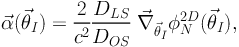
(4) |
The value of
depends on the local perturbation of the mass on space-time measured at
the location of
I.
The photon path follows a null geodesic that is
defined by ds2 = 0. Hence from Equation 3, one can
determine the travel time tT for a given path length
which in turn, is a function of the angle
. By
applying Fermat's principle, which states that light follows the path
with a stationary travel time, i.e. dtT /
dI =
 , we can
derive the value of the deflection
as a
function of the local Newtonian gravitational potential:
, we can
derive the value of the deflection
as a
function of the local Newtonian gravitational potential:
 |
(5) |
where φN2D is the Newtonian gravitational potential projected in the lens plane.
Combining Equations 4 and 5 we derive the lens equation under the thin lens approximation, which holds for a wide range of deflector masses, from stars to galaxies to clusters of galaxies (see Schneider, Ehlers & Falco 1992 for a more detailed derivation):
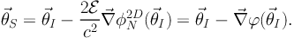 |
(6) |
The thin lens approximation is valid when the distances from the
observer to the lens and source are significantly larger than the
physical extent of the lens, an assumption that is strictly true for
all galaxies and clusters. Above we define ϕ as the lensing
potential - a lensing normalized version of the Newtonian projected
potential, and the distance ratio
 = DLS /
DOS which depends on the
redshift of the cluster zL and the background source
zS, as well as - but only weakly - on the cosmological
parameters Ωm and Ωλ. The
distance ratio measures the
efficiency of a given lens at redshift zL. The factor
is
an increasing function of the source redshift zS
(Figure 5); therefore the larger the background
source redshift, the stronger the deflection and distortion. This
relation can be slightly more complex for sources located in the strong
lensing regions. Note also that
is
independent of the Hubble constant, therefore lensing
deflection angles and deformations are independent of the value of
H0.
= DLS /
DOS which depends on the
redshift of the cluster zL and the background source
zS, as well as - but only weakly - on the cosmological
parameters Ωm and Ωλ. The
distance ratio measures the
efficiency of a given lens at redshift zL. The factor
is
an increasing function of the source redshift zS
(Figure 5); therefore the larger the background
source redshift, the stronger the deflection and distortion. This
relation can be slightly more complex for sources located in the strong
lensing regions. Note also that
is
independent of the Hubble constant, therefore lensing
deflection angles and deformations are independent of the value of
H0.
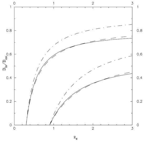 |
Figure 5. Lensing efficiency
|
It has also been shown that going beyond the thin lens approximation, the above lensing equation can be derived in the more general case (with Equation 4 being the limiting case for Einstein de-Sitter space-time) by simply calculating the null geodesics intersecting an observer's world-line without partitioning light paths into near and far lens regions (see Pyne & Birkinshaw 1996 for a detailed derivation). The particularly interesting case is when more than one lensing deflector is responsible for producing the observed magnification and shear. Observations suggest that the lensing effect of most clusters are likely further amplified due to the existence of multiple additional mass concentrations aligned along the line of sight. Therefore, multiple lens planes will ultimately need to be taken into account for accurate mass modeling of cluster lenses. The precise coupling between the lensing effects of two adjacent masses depends on their transverse separation. Examining the two-screen gravitational lens, Kochanek & Apostolakis (1988) find, albeit for galaxy-scale lenses, that their effects interact significantly for transverse separations less than 4 × r0 where r0 is the radius of the outer critical line of the singular potential. 4 Independent lenses that are close in redshift almost always interact and these interactions can lead to either an increase or a decrease in the total cross section relative to the cross section of two isolated lenses depending on the system's geometry. The resultant image geometries in such cases are dominated by the effects of fold caustics. The deflection can be calculated for the two-screen lens configuration numerically and most current lens equation solvers are adapted to do so.
2.3. Gravitational Lens Mapping
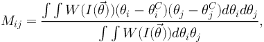
The effect of gravitational lensing can be modeled as a mathematical
transformation of source shapes into observed image shapes. The lensing
transformation is thus a mapping from the source plane (S) to the image
plane (I) [See Figure 6]. In the case of a
single lens plane, the Hessian of this transformation (also called the
magnification matrix) relates to first order a source element of the image
(dI) to the source plane
(dS) in the following way, in Cartesian and
polar coordinates, respectively:
 |
(7) |
This matrix is referred to as the magnification/amplification matrix and it is conventionally written as:
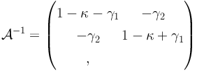 |
(8) |
where the convergence is defined as
κ = Δϕ / 2 = Σ / Σcrit and the
shear vector
(also often denoted as a complex number)
 =
(γ1, γ2) as:
=
(γ1, γ2) as:
 |
(9) |
and the norm is given by:
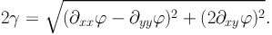 |
(10) |
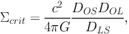
The term Σcrit is the critical lensing surface density defined as:
 |
(11) |
It can be clearly seen that the critical surface mass density scales as:
 |
(12) |
For instance, given a cluster lens at zL = 0.3 and a source at redshift zS = 1.0, DOS / DLS = 1.567 and (c / H0) / DOL = 4.661, yielding:
 |
(13) |
Thus, for a cluster with a depth of ∼ 300 kpc, the 3D mass density needed to reach the lensing critical surface mass density is about 10−24 g/cm3, which corresponds to a density that is ∼ 10,000 times the critical density of the Universe ρcrit. Background galaxies viewed via a cluster region where the surface mass density is critical or higher are likely to be multiply imaged.
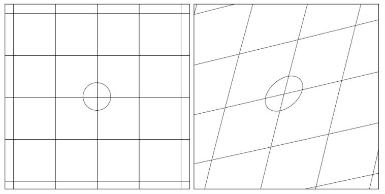 |
Figure 6. Illustration of the effect of lensing: local deformation of a regular grid and a circle (left: source map) by a lens with constant value of the convergence κ and the shear γ over the region (right: image map). |
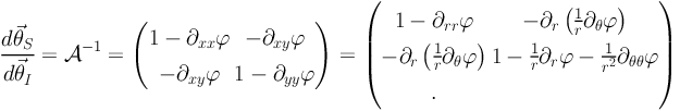
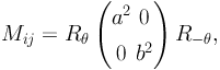
We can readily see that the magnification matrix is real and symmetric, therefore, it can be diagonalized, and can be written in its principal axes as follows:
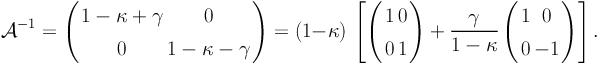 |
(14) |
From this equation, we see that 1 − κ describes the isotropic deformation, and the shear γ describes the anisotropic deformation. Note that the quantity that is most directly measured from faint galaxy shapes is the reduced shear g defined as: g = γ / (1 − κ).
The direction of the deformation (or equivalently of the shear) can be written as:
 |
(15) |
As the direction of the shear is a ratio of the components of the
lensing potential, the shear direction θshear will be
independent (modulo 90 degrees) of the distance ratio
= DLS /
DOS and thus will be independent of the source
redshift zS. Only the intensity or magnitude of the
shear will change with the source redshift zS.
2.4. Critical and caustic lines
The magnification µ is defined as the determinant of the magnification matrix and can be expressed as a function of κ and γ as:
 |
(16) |
The magnification is infinite if one of the principal values of the magnification matrix is equal to zero, which implies that the reduced shear g is equal to 1 or −1. Thus, the locus in the image plane of infinite magnification defines two closed lines that do not intersect (as g cannot be equal to 1 and −1 at the same location) and these are called the "critical lines". The corresponding lines in the source plane are called "caustic lines", they are also closed lines but contrary to the critical lines, they can intersect each other. In general, for a simple mass distribution, we can easily distinguish the two critical lines: the external critical line where the deformations are tangential, and the internal critical line where the deformations are radial. Note that these simple geometries for the critical and caustic lines do not hold strictly for more complex mass distributions (Figure 7 for examples of critical and caustic lines for different simple mass dsitributions).
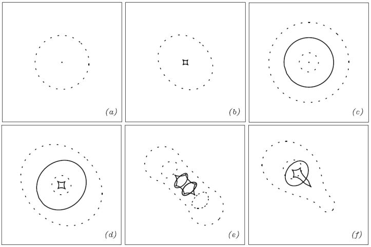 |
Figure 7. Critical lines (dashed) and caustics (solid) for different classes of mass models: (a) for a singular isothermal circular mass distribution, the radial critical line is the central point, and the corresponding caustic line is at infinity, (b) a singular isothermal elliptical mass distribution, the tangential caustic line is an astroid, (c) a circular mass distribution with an inner slope shallower than isothermal mass distribution, in this case a radial critical curve appears, and both caustics are circles. (d) same as (c) but for an elliptical mass distribution, the relative size of both caustic lines will depend on the mass profile and the ellipticity of the mass distribution, (e) a bimodal mass distribution with two clumps of equal mass, similar to (d), and (f) for a bimodal distribution with unequal masses. |
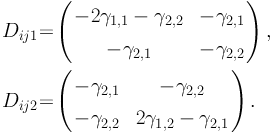
For a circularly symmetric mass distribution, the equations for the critical lines are simple. The magnification matrix in polar coordinates simplifies to:
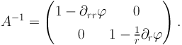 |
(17) |
Thus both the critical and caustic lines (if they exist) are circles. In fact, substituting the equation of the tangential critical line: r = ∂rϕ into the lensing equation to compute the caustic line, we find that the tangential caustic line is always restricted and reduces to a single point in the case of a circular mass distribution. It is also relatively easy to demonstrate that for a well behaved mass distribution the radial critical line is always located within the tangential critical line (Kneib 1993).
It is important to notice that for a circularly symmetric mass distribution, the projected mass enclosed within the radius r can be written as:
 |
(18) |
At the tangential critical radius we have: rct = ∂rϕ(rct), thus the mass within the tangential critical radius (also referred to as the Einstein radius rE) is:
 |
(19) |
The critical surface mass density Σcrit corresponds to the mean surface density enclosed within the Einstein radius. Thus the higher the mass concentration, the larger the Einstein radius. For a given surface mass density profile, the size of the Einstein radius will depend on the redshift of the lens and the source as well as the underlying cosmology. The variation of Σcrit for a given source redshift as a function of the lens redshift shows that for a given lens mass distribution the most effective lens is placed at roughly less than half the source redshift.
Furthermore, the radial critical curve is defined as:
 |
(20) |
thus, the position of the radial critical line depends on the gradient of the mass profile.
The above equations suggest that: i) from the tangential critical curve location, the total mass enclosed within a circular aperture can be measured precisely, and ii) from the radial critical curve, the slope of the mass profile near the cluster center can be strongly constrained. However, for an accurate estimate of the mass enclosed the redshifts of the cluster and the arc need to be known precisely. Furthermore, note that only the mass normalization scales directly with the value of H0, but not the derived mass profile slope.
 |
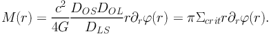
Figure 8. HST/ACS color image of MACSJ0451+00. The red curve shows the location of the critical line for a source at z = 2. A giant arc at z = 2.01, as well as different sets of multiple images are identified (each system of images is marked with a circle of the same color - the cyan and magenta identified multiple-image have no spectroscopic redshift measurement yet) [Richard et al. private communication]. |
For the general non-circular case, the determination of the critical lines cannot be addressed analytically except for certain simple elliptical mass profiles (e.g. Kneib 1993). The complexity of the shapes of critical lines can be seen for the lens model of MACS0451-02 (Figure 8). Indeed, to solve for the critical line in complex lens mass models, one has to resort to numerical methods. Iterative methods are more economical in terms of CPU time. For example, Jullo et al. (2007) have implemented the “Marching Square” technique for computing critical lines (see illustration in Figure 9).
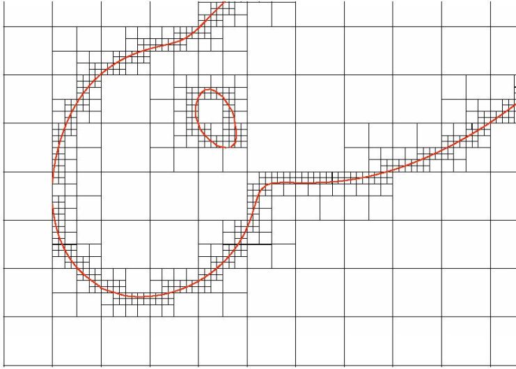 |
Figure 9. Multi-scale marching square field splitting to map critical lines: the boxes represent the splitting squares and the red lines chart the critical curve contour. The imposed upper and lower limits for the box sizes are 10” (corresponding to the largest box shown) and 1” respectively. The 1” boxes are not plotted here for clarity. Figure adapted from Jullo et al. (2007) where more details may be found. |
The above property linking the total mass within the critical line to the area within the critical line does not hold exactly for the more general cases but it is still a good approximation if the mass distribution is not too different from the circularly symmetric case (Kassiola & Kovner 1993). Hence identifying the characteristic sizes of the critical lines both radial and tangential in an observed cluster is the first important step toward measuring the mass and its degree of concentration in the inner regions.
Critical lines are virtual lines, and thus cannot be directly mapped. However, multiple-images that straddle critical lines can easily be identified in high resolution images. For instance, tangentially distorted images are found near tangential critical lines and radially distorted ones near the radial critical lines. One often refers to tangential pairs or radial pairs, which are simple configurations that are easily recognizable (e.g. Miralda-Escude & Fort 1993). For example, one can have triplets, quadruplets, quintuplets or even larger multiplicities of images of the same source depending on the complexity of the mass distribution.
The number of multiple-images produced is simply the number of solutions of Equation 6. It can be estimated easily using catastrophe theory (Thom 1989, Zeeman 1977, Erdl & Schneider 1993), according to which each time one crosses a caustic line in the source plane two additional lensed images are produced. For a non-singular mass distribution we expect to always have an odd number of multiple-images (Burke 1981). However, some images are likely to be less magnified, or in fact, demagnified so that they are not observable, thereby complicating at first the task of counting the total number of multiple-images produced. Often, the presence of a bright central galaxy in clusters scuppers the detection of the central demagnified image.
2.5.2. Multiple-image symmetry
Multiple-images have different symmetries which can be summarized by the signs of the eigenvalues of the magnification matrix, we can thus in principle have three possibilities for the parities, which correspond to the symmetry of the source, denoted as: (+,+), (+,-) and (-,-). For example we often talk about “mirror” symmetry, when we recognize a counter image as the flipped image of galaxy with a remarkably similar morphology. The image symmetry property is generally used to identify multiple-images in what turns out to be a secure way, as we see in the pair configuration of Figure 13.
Indeed, each time, one crosses a critical line (this corresponds to a change in sign of one of the eigenvalues of the magnification matrix), the parity of the image changes (Blandford & Narayan 1986; Schneider, Ehlers & Falco 1992). For simple mass distributions, only three parities described above by the notation (+,+), (-,-) and (+,-) can be observed as shown in Figure 10. Since for a simple mass distribution the radial critical line is always inside the tangential critical line, the parity (-,+) is not physically allowed.
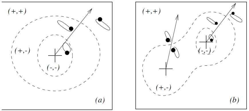 |
Figure 10. Area in the image plane showing different image parities (indicated by the signs in parentheses): (a) in the case of a simple elliptical mass distribution, (b) in the case of a bimodal mass distribution. The dashed lines correspond to the critical lines. The arrow is just an indication of the radial direction of the closest mass clump. We note that while the deformations shown in this figure are completely arbitrary, the orientation of the images is portrayed accurately. |
2.5.3. Examples of multiple-image systems
Massive clusters frequently produce multiple-images, and this happens when the surface mass density of the cluster core is close to or larger than the critical surface mass density:
 |
for given lens and source redshifts. The detailed configuration of multiple-images can be used to unravel the structure of the mass distribution.
A cluster with one dominant clump of mass will produce (for the range of multiple-image configurations see Figure 11) fold, cusp or radial arcs (e.g MS2137.3-2353: Fort et al. 1992, Mellier et al. 1993; AC114: Natarajan et al. 1998; A383: Smith et al. 2001, 2003); a bimodal cluster can produce straight arcs (e.g A2390: Pelló et al 1991, Cl2236-04: Kneib et al. 1994), triplets (A370: Kneib et al. 1993, Bezecourt et al. 1999); a very complex structure with lots of massive halos in the core can produce multiple-image systems with 7 or more images of the same source (e.g A2218, see Figure 12). The presence of every nearby perturbing mass can typically add two extra images to a simple configuration if that mass is well positioned relative to the central core. Very elongated/elliptical clusters with appropriate inner density profile slopes can produce hyperbolic-umbilic catastrophes producing quintuple arc configurations such as the one seen in Abell 1703 (Limousin et al. 2008). A thorough description of exotic configurations has been discussed quite extensively in a paper by Orban de Xivry & Marshall (2009).
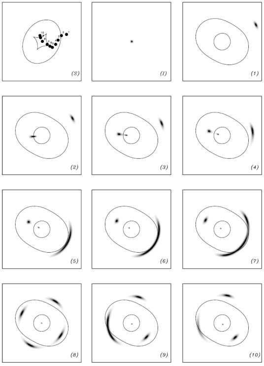 |
Figure 11. Multiple-image configurations produced by a simple elliptical mass distribution. The panel (S) shows the caustic lines in the source plane and the positions numbered 1 to 10 denote the source position relative to the caustic lines. The panel (I) shows the image of the source without lensing. The panels (1) to (10) show the resulting lensed images for the various source positions. Certain configurations are very typical and are named as follows: (3) radial arc, (6) cusp arc, (8) Einstein cross, (10) fold arc. |
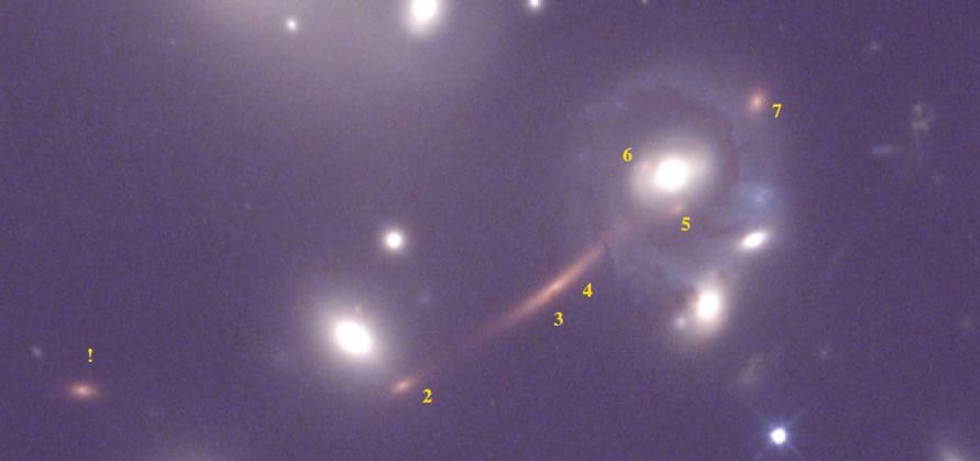 |
Figure 12. A spectacular set of multiple-images seen in the cluster Abell 2218 in the composite B, R, and I-band HST image. A distant E/S0 galaxy at z = 0.702 is lensed into a 7-image configuration. |
2.5.4. Multiple-image identification
Multiple-images can be identified by their distinct properties. Traditionally, multiple-images have been recognized as the images forming the giant arcs (3 images in the case of Abell 370, but only two images in the case of MS2137-17 or Cl2244-04). However, not every giant arc is composed of multiple-images, for example it is most likely that the northern giant arc in Abell 963 is only a single image, and that the southern arc in Abell 963 is composed of two or three arclets (single images) from sources at different redshifts as revealed by their different colors. Multiple-images can be recognized in terms of their (mirror) symmetry, which is of course best visible with high-resolution HST data. One of the classic examples is the “hook-pair” in AC114 (Figure 13) where the image symmetry is readily identified. Furthermore, as lensing is achromatic, multiple-images can be recognized by the similarity of their colors, or by their extreme brightness at a specific wavelength like in the sub-mm or in mid-infra red.
 |
Figure 13. The lensed pair S1-S2 in AC114. This galaxy at z = 1.867 displays the surprising morphology of a hook, with an obvious change in parity (Smail et al 1995a, Campusano et al 2001). |
Finally, the secure way to identify and confirm the existence of a multiple-image system, is through the detailed modeling of the cluster lens itself. This allows one in principle to test if a set of images having similar morphology and colors can actually be multiple images of the same source. Calibrated lens models can predict the location of counter images and also predict the redshift of the multiply lensed source (Kneib et al. 1993, 1996).
Ultimately, for studying a large sample of massive clusters, one would likely need to develop automatic techniques to identify multiple-image systems based on their morphology, color and more sophisticated lens modeling software. Although such robotic processes are being developed (Sharon private communication), further developments are needed to make them completely user friendly.
Multiple-images are located in the central regions of clusters where the surface mass density is close to or higher than the lensing critical surface density. For a given source redshift one can compute the region conducive to multiple-imaging and the expected multiplicity. This is easily computed, as for any given image position θI, we can determine the source position θS using the lensing equation (Equation 4). Given a source position it is straightforward to determine whether θS lies within a caustic curve or not. The expected number of images is given by (1 + 2 Nc) where Nc is the minimum number of caustic curves that need to be crossed to reach the position θS (Figure 14). The calculation of multiple-imaging regions can be useful to help observationally identify multiple-image counterparts (Figure 15) particularly in the case of complicated mass distributions.
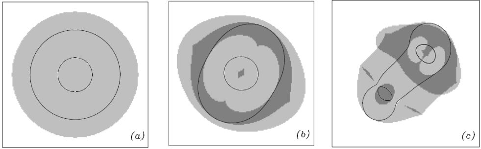 |
Figure 14. Diagram showing the regions wherein multiple-images are produced with the location of critical lines marked, for the case of different mass models (a) circular mass distribution; (b) an elliptical mass distribution and (c) a bimodal mass distribution. The grey scale areas indicate regions behind which we can expect a single background galaxy to be imaged into three (light grey) or five (dark grey) multiple-images. |
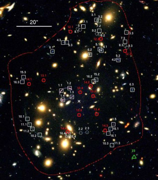 |
Figure 15. Hubble ACS color image of Abell 1703 (image shown is from the combination of the F450W, F606W and F850LP filters), showing the location of all the multiply imaged systems. The white cross at the center of the image marks the location of the brightest cluster galaxy, which has been subtracted from this image for clarity. The red dashed line outlines the limit of the region where we expect multiple-images from sources out to z = 6 (Figure from Richard et al. 2009). |
2.6. First order shape deformations - Shear
Distant sources are only multiply imaged in the central regions of cluster where the surface mass density is sufficiently high. However, every observed galaxy image in the field of the cluster is deformed by lensing, typically in the weak regime. To first order, one can approximate the light distribution of a galaxy as an object with elliptical isophotes. In this event, the shape and size of galaxies can be defined in terms of the axis ratio and the area enclosed by a defined boundary isophote.
However, the real shapes of faint galaxies can be quite irregular and not
well approximated by ellipses. We thus need to express the shape of a
galaxy in terms of its pixelized surface brightness as measured on a
digital detector. For this purpose, we use the moments of the
light distribution to define shape parameters. If
I()
is the surface brightness distribution of the galaxy under
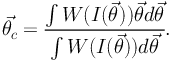
consideration, we can define the center of the image
c
= (iC,
jC) using the first moment of the
I()
distribution:
 |
(21) |
Note that W(I) is a weight/window function, that allows the integrals
above to be finite in the case of noisy data. The simplest choice for the
function W(I) is the heaviside step function
H(I − Iiso) which is equal to 1 for
I(
> Iiso where Iiso is the
isophote limiting the detection of the object, and 0 otherwise. The image
center found is then taken as the center of the detection isophote. Another
popular weight function that is frequently adopted is:
W(I) = I × H(I −
Iiso), where the window function is now weighted by
the light distribution within the isophote.
The second order moment matrix of the light distribution centered on
c:
 |
(22) |
allows us to define the size, the axis ratio and the orientation of the corresponding approximated ellipse. Indeed the moment matrix M is positive definite and can be written in its principal axes as:
 |
(23) |
where a and b are the semi-major and semi-minor axes respectively, and θ the position angle of the equivalent ellipse, and Rθ is the rotation matrix of an angle θ. Thus the moment matrix M contains three parameters: the size of the galaxy, its ellipticity and its orientation (see illustration in Figure 16)
 |
Figure 16. A typical faint galaxy observed on a CCD image (left), and the equivalent ellipse defined from the second order moments (right). |
It is useful to define a complex ellipticity which encodes both the shape parameter and the orientation of an observed galaxy.
There are however a number of ways to define the norm of the complex ellipticity, and the lensing community has experimented several notations:
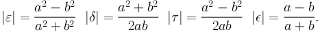 |
(24) |
With the complex ellipticity defined for example as:
 |
(25) |
The notation є was the first to be introduced, as it emerges naturally from the moment calculation, then τ and δ were introduced in the context of cluster lensing by Kneib (1993) and Natarajan & Kneib (1997). The advantage of this form is that the lens mapping can be written as a simple linear transformation from the image plane to the source plane which is mathematically convenient. Subsequently є was adopted, and it has now become the standard definition, essentially because it is a direct estimator (modulo the PSF correction) of the measured quantity, which is the reduced shear g as we show below. All ellipticity parameters are of course linked to each other, and in particular we have є = 2є / (1 + |є|2).
With the various definitions in hand for the relevant parameters, we
can now explicitly express the transformation produced by
gravitational lensing on the shape of a background galaxy. First,
it can be shown that the image
of the center of the source corresponds to the center of the image in
the case where the magnification matrix does not change significantly
across the size of the image
(Kochanek 1990;
Miralda-Escude 1991).
This is generally adopted as the definition
of the weak lensing regime as such a simplification does not hold in the
strong lensing regime. To demonstrate this explicitly, one has to use the
fact that the surface brightness is conserved by gravitational lensing
as was first demonstrated by
Etherington (1933),
namely,
I(I) =
I(S).
The lens mapping will transform the shape of the galaxy, by magnifying it and stretching it along the shear direction. This transformation can be written in terms of the moment matrix MS (for the galaxy in the source plane) and MI (for the galaxy in the image plane that is, as observed) as follows:
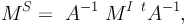 |
(26) |
or if the matrix A−1 is not singular:
 |
(27) |
Note that t A is the transpose of matrix A.
These equations describe how the ellipse defining the source shape is mapped onto the equivalent ellipse of the image or vice versa. If we consider the size σ = π a × b of the equivalent ellipse, we can write:
 |
(28) |
Thus the overall size σS of the source is enlarged by the magnification factor µ. Similarly, it is possible to write the lensing transformation for the complex ellipticity, which of course will depend on the ellipticity estimator chosen. For the ellipticity є, and using the complex notation, we have:
 |
(29) |
which corresponds to the region external to the critical lines, and
 |
(30) |
which corresponds to the region inside the critical lines (the notation * denotes the transpose of a complex number).
In the weak regime, where the distortions are small (|g| << 1) the lensing equation simplifies to:
 |
(31) |
Thus the ellipticity of the image is just a linear sum of the intrinsic source ellipticity and the lensing distortion in this limit. Thus averaging the above equation over a number of sources yields the convenient fact that image ellipticities are a direct measure of the reduced shear g. Note, however that these simplified equations mask observational limitations such as the PSF/seeing convolution and pixelization, all effects that contribute to and contaminate observed image shapes.
The "mass sheet degeneracy" problem was recognized as soon as mass distributions began to be mapped using lensing observations (e.g. Falco et al. 1985) and the issue has been discussed in detail in Schneider, Ehlers & Falco (1992) and Schneider & Bartelmann (1997) and Bradač et al (2004) in the context of weak lensing mass measurement. This degeneracy arises due to the lack of information needed to calibrate the total mass of clusters in the absence of a normalization scheme due to the simple fact that the addition of a constant surface mass density sheet leaves the measured shear unaltered.
Expressed mathematically, the magnification and shear are invariant under the following transformation:
 |
(32) |
and
 |
(33) |
where λ is the mass-sheet (denoting a sheet of constant surface mass density) added to the lens plane. Expressing the reduced shear with the above two equations we can show that:
 |
(34) |
thus the reduced shear is conserved under this transformation. This means that for a given observed reduced shear field, one can only extract the surface mass density distribution κ up to a constant factor given by the unknown value of λ.
There are several ways to break the mass sheet degeneracy, the
obvious way is to use lensed sources from different source redshift
planes. Indeed with, κ(z1) =
(z1) /
(z2)
κ(z2), such a transformation is incompatible
with the above invariance. Other methods to break the mass-sheet
degeneracy, such as the inclusion of constraints from the strong lensing
regime are discussed further in
Section 3.4.3 on lens modeling.
2.8. Higher order shape deformations - Flexion
The equations in the previous section assume that κ and γ and as a consequence the reduced shear g are all constant across an image. This assumption fails when an image is physically large and/or when it is close to critical regions where the lensing distortion is changing rapidly. There are basically two effects that lensing produces on a background elliptical source: a shift in the peak flux at the center of the image compared to that of the fainter isophotes (while still preserving the surface brightness from the source to the image), and the distortion of the elliptical shape into an extended "banana" shape. Therefore, there is additional, valuable information that can be gleaned from higher order lensing effects.
To determine these higher order effects numerically, one needs to use higher orders of the lensing transformation using the Taylor expansion of the image shape. This was first investigated by Goldberg & Natarajan (2002), and followed up by Goldberg & Bacon (2005). A recent summary of the formalism and applications is reviewed in Bacon et al. (2005). Flexion is the significant third-order weak gravitational lensing effect responsible for the skewed and arc-like appearance of lensed galaxies. Flexion has two components: the first flexion, which is essentially the derivative of the shear field which contains local information about the gradient of the matter density (Goldberg & Natarajan 2002) and the second flexion which contains non-local information (Bacon et al. 2005 and Figure 17). Flexion measurements can be used to measure density profiles and these reconstructions can be combined with those derived from the shear alone. One key advantage of using the flexion estimator is that it is not plagued by the mass sheet degeneracy as it is a higher order term, while its dispersion measure is comparable to that of the shear. Recent successful applications of flexion to map mass distributions can be found in Okura et al. (2008); Leonard, King & Goldberg (2011) and Er, Li & Schneider (2011).
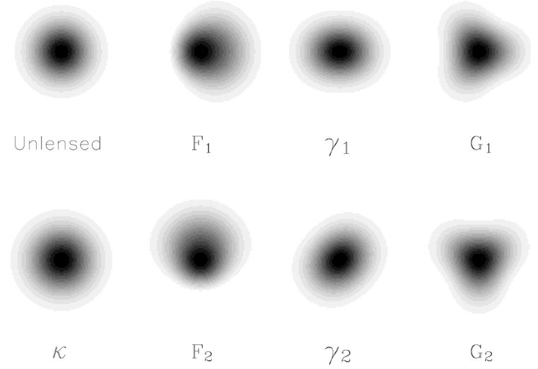 |
Figure 17. Decomposition of weak lensing distortions, illustrated for an unlensed Gaussian galaxy with a radius of 1 arcsec. The source has been distorted with 10% convergence/shear, and 0.28 arcsec−1 flexion. The convergence κ, and two components of the first flexion (F1 and F2); shear (γ1, γ2); and second flexion G1 and G2 are shown. As mentioned, flexion causes the arci-ness or elongation of weakly lensed arcs once one combines F, G and γ (Figure from Bacon et al. 2005). |
The shear and convergence vary within a galaxy image, flexion is the higher order derivative and in order to derive it, expansion to the second order is required:
 |
(35) |
with
 |
(36) |
Using results from Kaiser (1995), we find that
 |
(37) |
Using the equations above, the surface brightness of the imagecan be expanded in a Taylor series. In the weak lensing regime we can approximate the brightness to second order as follows:
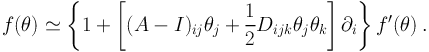 |
(38) |
Therefore the expression for flexion can be written in terms of derivatives of the shear field. Using the notation of Kaiser (1995) we can write flexion in terms of the gradient of the convergence:
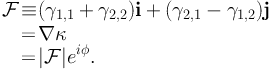 |
(39) (40) (41) |
We need to be able to measure the derivatives of the shear field γi,j with a high degree of accuracy from images in order to measure flexion. This is becoming γi,j with sufficient accuracy. This is becoming increasingly feasible with the availability of high quality imaging data. The first flexion probes the local density via the gradient of the shear field and quantifies the variation of the center of the different isophotal contours. The second flexion probes the nonlocal part of the gradient of the shear field and quantifies the shape variation and departure from elliptical symmetry.
Flexion has been incorporated as an additional constraint in the cluster mass reconstructions only recently as extremely high quality data is required to extract the flexion field and this is very challenging (see Leonard, King & Goldberg 2011 for the case of Abell 1689). This higher order shape estimator however offers a powerful probe provided it can be measured accurately from observations (Leonard & King 2010; Er, Li & Schneider 2011). As an illustration, we present the calculation of the flexion for the SIS model in the Appendix (A.4).
4 Critical lines and caustics are defined in the next subsection. Back.