


Following their discovery, the first important step in clarifying the nature of the UFDs was to determine their stellar velocity dispersions. By measuring the velocities of individual stars in several systems, these early studies constrained their dynamical masses and dark matter content.
The initial spectroscopic observations of UFDs were made by Kleyna et al. (2005) for Ursa Major I (UMa I) and Muñoz et al. (2006) for Boötes I (Boo I). Using Keck/HIRES spectra of 5 stars, Kleyna et al. measured a velocity dispersion of σ = 9.3−1.2+11.7 km s−1. Muñoz et al. determined a velocity dispersion of σ = 6.6 ± 2.3 km s−1 from WIYN/Hydra spectra of 7 Boo I stars. These two systems have luminosities of 9600 and 21900 L⊙, respectively. If the stellar mass-to-light ratio is ≈ 2 M⊙ / L⊙ (as expected for an old stellar population with a standard initial mass function), then the expected velocity dispersions from the stellar mass alone would be ≲ 0.1 km s−1 (making use of the Wolf et al. (2010) mass estimator). In both cases, such a small velocity dispersion can be ruled out at high significance, demonstrating that under standard assumptions UFDs cannot be purely baryonic systems. Similar conclusions quickly followed for the remaining ultra-faint dwarfs based on analyses of Keck/DEIMOS spectroscopy by Martin et al. (2007) and Simon & Geha (2007). At the present, velocity dispersion measurements or limits have been obtained for 27 out of 42 confirmed or candidate UFDs. All of the available kinematic data are displayed in Figure 3.
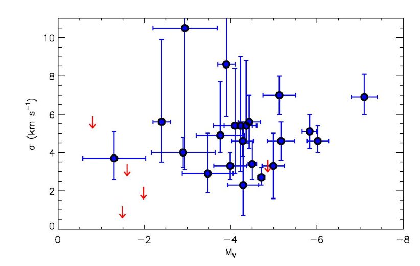 |
Figure 3. Line-of-sight velocity dispersions of ultra-faint Milky Way satellites as a function of absolute magnitude. Measurements and uncertainties are shown as the blue points with error bars, and 90% confidence upper limits are displayed as red arrows for systems without resolved velocity dispersions. The dwarf galaxy data included in this plot are listed in Table 1. Although there is a clear trend of decreasing velocity dispersion toward fainter dwarfs among the classical dSphs, in the ultra-faint luminosity regime there is much more scatter and any systematic trend is weak. |
2.1. Mass Modeling and Dark Matter Content
2.1.1. Assumptions Required for Determining Masses. The results shown in Figure 3 are simply measurements: the observed dispersion of the radial velocities for the set of stars in each dwarf for which spectra were obtained. In order to translate these velocity dispersions into dynamical masses, several assumptions must be made. First, no inference can be drawn about the mass of a system unless it is in dynamical equilibrium. If a dwarf galaxy has experienced, for example, a recent tidal shock, then its present velocity dispersion may not be a reliable indicator of its mass. Recent proper motion measurements show that many of the ultra-faint dwarfs are indeed close to their orbital pericenters, but those pericentric passages occur at typical distances of nearly 40 kpc away from the Galactic center, lessening their impact (Simon, 2018). While the assumption of equilibrium deserves further attention in modern high-resolution simulations, earlier studies indicate that even when dwarf galaxies have been tidally disturbed their velocity dispersions do not change substantially, and the instantaneous dispersion remains a good barometer of the bound mass (Oh, Lin & Aarseth, 1995, Piatek & Pryor, 1995, Muñoz, Majewski & Johnston, 2008).
Second, unless spectroscopy of a dwarf is obtained over multiple, well-separated observing runs, it must be assumed that binary stars are not inflating the observed velocity dispersion above its true value. The influence of binary stars may be particularly concerning given the recent suggestion that the binary fraction is quite large at low metallicities (Moe, Kratter & Badenes, 2018). Several individual binary stars have been detected in UFDs (e.g., Frebel et al., 2010, Koposov et al., 2011, Koch et al., 2014, Ji et al., 2016c, Kirby et al., 2017, Li et al., 2018b), and the binary population of Segue 1 was evaluated statistically by Martinez et al. (2011) and Simon et al. (2011). Only the binary system in Hercules identified by Koch et al. (2014) has an orbit solution (with period 135.28 ± 0.33 d and velocity semi-amplitude 14.48 ± 0.82 km s−1), but the few other UFD binaries with detected velocity variability appear to have semi-amplitudes of ∼ 10−20 km s−1 and periods ≲1 yr as well (Ji et al., 2016c, Kirby et al., 2017, Li et al., 2018b). Frebel, Simon & Kirby (2014) also found indirect evidence of binarity for a star in Segue 1 based on its chemical abundances, which are best explained by mass transfer from a (formerly) more massive companion star.
In the classical dSphs, a number of studies have shown that binary stars do not significantly inflate the observed velocity dispersions (e.g., Olszewski, Aaronson & Hill, 1995, Olszewski, Pryor & Armandroff, 1996, Vogt et al., 1995, Hargreaves, Gilmore & Annan, 1996, Kleyna et al., 2002, Minor et al., 2010, Spencer et al., 2017). It has also been suggested, however, that the effect of binaries may be larger in UFDs given their smaller intrinsic velocity dispersions (McConnachie & Côté, 2010, Spencer et al., 2017). While that is certainly true in principle, observationally most UFD data sets do not seem to be significantly affected by binaries. For example, removing the radial velocity variables from the sample of Boo I stars analyzed by Koposov et al. (2011) changes the velocity dispersion by only ∼ 3%. 3 Similarly, Martinez et al. (2011) and Simon et al. (2011) corrected the effects of binaries in Segue 1 with Bayesian modeling of a multi-epoch radial velocity data set and found that the binary-corrected velocity dispersion agrees within the uncertainties with the uncorrected dispersion. Other recent studies have also included multi-epoch velocity measurements, either finding no obvious binaries (Simon et al., 2017) or removing the binaries before computing velocity dispersions (Li et al., 2018b). On the other hand, there are at least two examples of binary stars indeed biasing the derived velocity dispersions of UFDs: Ji et al. (2016c), Venn et al. (2017), and Kirby et al. (2017) showed that Boötes II (Boo II) and Triangulum II (Tri II) each contain a bright star in a binary system that was responsible for substantially increasing the velocity dispersions determined by Koch et al. (2009) for Boo II and by Martin et al. (2016b) and Kirby et al. (2015) for Tri II. In both of these cases, the influence of the binary was magnified by the very small samples of radial velocities available (5 stars in Boo II and 6−13 stars in Tri II). These results indicate that while binary stars do not significantly change the velocity dispersions of most ultra-faint dwarfs, studies consisting of single-epoch velocity measurements of small numbers of stars should be interpreted with caution.
Finally, an often unstated assumption is that samples of ultra-faint dwarf member stars are free from contamination by foreground Milky Way stars. Contamination is a particularly tricky issue for galaxies with velocities close to the median velocity of Milky Way stars along that line of sight (e.g., Willman 1, Hercules, and Segue 2 4), although incorrectly identified members are possible in any dwarf. Because stars that could be mistaken for UFD members must have velocities close to the systemic velocity of the dwarf, the effect of such contaminants is likely more severe for the derived metallicity distribution than the velocity dispersion (e.g., Siegel, Shetrone & Irwin, 2008, Kirby et al., 2017). Several examples of erroneously determined UFD members are available in the literature. Simon (2018) demonstrated that stars previously classified as members of Ursa Major I (UMa I) by Kleyna et al. (2005) and Simon & Geha (2007) and Hydrus I (Hyi I) by Koposov et al. (2018) have Gaia proper motions that strongly disagree with the remaining members. Removing these stars from the member samples reduces the UMa I velocity dispersion from 7.6 ± 1.0 km s−1 to 7.0 ± 1.0 km s−1 and has no effect on the measured dispersion of Hyi I. Similarly, Frebel et al. (2010) obtained a high-resolution spectrum of a star identified by Simon & Geha (2007) as an Ursa Major II (UMa II) member but found that its surface gravity was not consistent with that classification; the velocity dispersion of UMa II is not significantly changed by the exclusion of this star. Adén et al. (2009) argued using Strömgren photometry that the Hercules member sample from Simon & Geha (2007) was contaminated by several non-member stars, but the derived velocity dispersions are only 1.1σ apart.
For the classical dSphs, where large member samples of hundreds to thousands of stars are generally available, a common method for dealing with foreground contamination is to make use of membership probabilities for each star (e.g., Walker et al., 2009b, Caldwell et al., 2017). These probabilities are determined via a multi-component model of the entire data set, e.g., assuming Gaussian velocity and metallicity distributions and a Plummer (1911) radial profile for the dwarf galaxy. The global properties of the dwarf can then be computed using the individual membership probabilities as weights, with a star with a membership probability of 0.5 counting half as much as a certain member with a probability of 1.0. In the limit where there are many stars with intermediate membership probabilities (0.1 ≲ pmem ≲ 0.9), some of which are genuine members and some of which are foreground stars, the reduced contributions of actual members and the increased contributions of contaminants can reasonably be assumed to cancel out so that the derived properties of the system are accurate. It is less clear, however, that this statistical approach works well when applied to the small data sets typical for UFDs. For example, the stars with ambiguous membership status are likely to be those that are outliers from the remainder of the population in velocity and/or metallicity. In reality, of course, each such star is either a member of the dwarf or not. If there is only a single star in this category, probabilistically including it as, say, 0.5 member stars may substantially change the inference on the velocity or metallicity dispersion of the system. In the shot noise-limited regime, a better approach to deal with outliers may be simply to report the derived values with and without the questionable star(s) included, acknowledging the resulting uncertainty. Fortunately, the advent of Gaia astrometry should make it possible to correctly classify most stars whose membership would previously have been uncertain, reducing the importance of this issue going forward.
2.1.2. Dynamical Masses and Dark Matter. Once the assumptions of dynamical equilibrium and minimal contamination by binary stars and foreground stars are made, the observed velocity dispersion can be used to constrain the mass of a dwarf galaxy. Early work (e.g., Kleyna et al., 2005, Muñoz et al., 2006, Martin et al., 2007, Simon & Geha, 2007) relied on the method of Illingworth (1976) for determining globular cluster masses, as applied by Mateo (1998) to dSphs. The Illingworth formula is based on the dynamical model developed by King (1966), again for globular clusters. As discussed by Wolf et al. (2010), several key assumptions of this method fail (or may fail) in the case of dwarf galaxies. In order of increasing severity, these assumptions include that (1) the velocity dispersion is independent of radius, (2) the velocity dispersion is isotropic, and (3) the mass profile follows the light profile. An alternate formalism is therefore needed; in particular, one in which the mass is not assumed to be distributed in the same way as the light.
Wolf et al. (2010) showed that for dispersion-supported stellar systems with unknown velocity anisotropy, the mass that is most tightly constrained by stellar velocity measurements is the mass enclosed within the three-dimensional half-light radius of the system, M1/2 = M(< r1/2,3D). This approach still requires that the velocity dispersion profile be approximately flat in the measured region (which is generally the case in the dwarf galaxies for which that measurement can be made), but does not assume anything about the shape of the anisotropy profile or the mass distribution. According to Wolf et al. (2010),
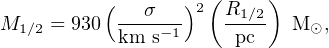 |
(1) |
where σ is the velocity dispersion and R1/2 is the projected two-dimensional half-light radius. 5 (One can also write this relation in terms of the deprojected three-dimensional half-light radius, r1/2, but that is less convenient since R1/2 is what can be measured directly. For many light profiles the two are simply related by r1/2 = 4/3R1/2, as shown by Wolf et al. (2010).)
The dynamical masses determined with Equation 1 are displayed in Figure 4. Every UFD for which the velocity dispersion has been measured has a mass of at least 105 M⊙ within its half-light radius. Among the five systems with only upper limits on the dispersion available, all but Tucana III (Tuc III) are consistent with such masses as well. In comparison, the luminosities are a factor of ∼ 100 or more smaller. Given that the stellar mass-to-light ratio is ∼ 2 M⊙ / L⊙ for an old stellar population with a Salpeter (1955) initial mass function 6 (e.g., Martin, de Jong & Rix, 2008), it is clear that nearly all of the UFDs have masses that are dominated by something other than their stars.
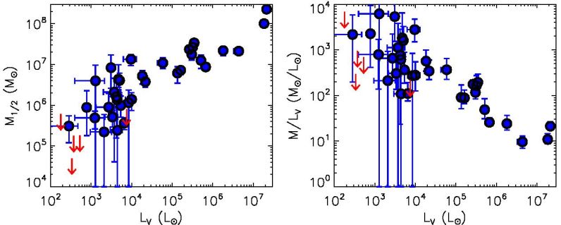 |
Figure 4. (left) Dynamical masses of ultra-faint Milky Way satellites as a function of luminosity. (right) Mass-to-light ratios within the half-light radius for ultra-faint Milky Way satellites as a function of luminosity. Measurements and uncertainties are shown as the blue points with error bars, and mass limits determined from the 90% confidence upper limits on the dispersion are displayed as red arrows for systems without resolved velocity dispersions. The dwarf galaxy/candidate data included in this plot are listed in Table 1. |
2.1.3. Galaxies for which Published Kinematics May Not Reliably Translate to Masses. The reported stellar kinematics and corresponding masses of UFDs often seem to be regarded as having uniform reliability, especially by those other than the original observers. In fact, however, there are wide variations from galaxy to galaxy in how well determined the internal kinematics are. The size of the member sample, the quality of the individual velocity measurements, and the evolutionary history of the object in question all influence the degree to which accurate dynamical inferences can be made. Some specific objects that should be treated with caution include:
2.2. Identification as Galaxies
Prior to the discovery of dwarf galaxies fainter than MV ∼ −5, dwarfs and globular clusters occupied distinct and cleanly separated portions of the size-luminosity parameter space displayed in Fig. 2. Consequently, there was little discussion of whether certain objects should be considered to be galaxies or clusters; the classification of all known systems was obvious. 7
As the dwarf galaxy population grew toward lower luminosities and smaller radii, the gap between dwarfs and globular clusters in the size-luminosity plane disappeared, such that size alone was no longer sufficient to determine the nature of an object. Conn et al. (2018) dubbed the region occupied by a number of ultra-faint satellites (14 < r1/2 < 25 pc) the “trough of uncertainty” to emphasize the difficulty in classifying these systems. In order to resolve the confusion caused by the lack of an agreed-upon system for separating galaxies from star clusters, Willman & Strader (2012) proposed the following definition:
“A galaxy is a gravitationally bound collection of stars whose properties cannot be explained by a combination of baryons and Newton’s laws of gravity.”
Applied to UFDs, this definition is generally interpreted as requiring an object to have either a dynamical mass significantly larger than its baryonic mass or a non-zero spread in stellar metallicities to qualify as a galaxy. The former criterion directly indicates the presence of dark matter (for which there is no evidence in globular clusters), while the latter indirectly suggests that the object must be embedded in a dark matter halo massive enough that supernova ejecta can be retained for subsequent generations of star formation.
The early SDSS UFDs were all measured to have velocity dispersions larger than 3 km s−1, implying that they are composed mostly of dark matter and can be straightforwardly classified as galaxies (Kleyna et al., 2005, Muñoz et al., 2006, Martin et al., 2007, Simon & Geha, 2007, Geha et al., 2009). Some disagreement persisted for several years regarding the nature of the two least-luminous systems, Willman 1 and Segue 1 (e.g., Belokurov et al., 2007, Siegel, Shetrone & Irwin, 2008, Niederste-Ostholt et al., 2009), but ultimately the combination of stellar kinematics, metallicities, and chemical abundance measurements led to the conclusion that both are dwarfs (Willman et al., 2011, Simon et al., 2011, Frebel, Simon & Kirby, 2014). The first object for which kinematic classification failed entirely was Segue 2. Despite a comprehensive analysis of the kinematics of Segue 2, Kirby et al. (2013a) were unable to measure its velocity dispersion, finding σ < 2.6 km s−1 at 95% confidence. With only an upper limit on the dynamical mass and mass-to-light ratio, it cannot be confirmed that Segue 2 contains dark matter. However, Kirby et al. also showed that the stars of Segue 2 span a large range of metallicities, from [Fe/H] = −2.9 to [Fe/H] = −1.3, with a dispersion of 0.43 dex. Segue 2 can therefore still be classified as a galaxy rather than a globular cluster on the basis of its chemical enrichment.
The discovery of larger numbers of compact ultra-faint satellites in Dark Energy Survey and Pan-STARRS data (Bechtol et al., 2015, Koposov et al., 2015a, Drlica-Wagner et al., 2015, Laevens et al., 2015b, 2015a) has increased the difficulty in classification. For several of these objects only upper limits on the velocity dispersion have been obtained (Kirby, Simon & Cohen, 2015, Kirby et al., 2017, Martin et al., 2016a, Simon et al., 2017), and in the case of Tuc III no metallicity dispersion is detectable in current data either (Simon et al., 2017). In such situations one must either accept the uncertainty in the nature of some systems or rely on more circumstantial arguments such as size, survival in a strong tidal field (e.g., Simon et al., 2017), mass segregation (Kim et al., 2015b), or chemical peculiarities .
As of this writing, the following 21 satellites can be regarded as spectroscopically confirmed ultra-faint dwarf galaxies: Segue 2, Hydrus 1, Horologium I, Reticulum II, Eridanus II, Carina II, Ursa Major II, Segue 1, Ursa Major I, Willman 1, Leo V, Leo IV, Coma Berenices, Canes Venatici II, Boötes II, Boötes I, Hercules, Pegasus III, Aquarius II, Tucana II, and Pisces II. Satellites that may be dwarfs but for which either no spectroscopy has been published or the data are inconclusive include: Tucana IV, Cetus II, Cetus III, Triangulum II, DES J0225+0304, Horologium II, Reticulum III, Pictor I, Columba I, Pictor II, Carina III, Virgo I, Hydra II, Draco II, Sagittarius II, Indus II, Grus II, Grus I, Tucana V, Phoenix II, and Tucana III. The most extended of these objects, such as Tucana IV, Cetus III, Columba I, and Grus II, are perhaps the most likely to be dwarfs given their large radii. We have not included Boötes III, which is likely the remnant of a dwarf, in either category because it is not clear whether it is still a bound object (Grillmair, 2009, Carlin et al., 2009, Carlin & Sand, 2018).
The problem of determining the nature of the faintest and most compact Milky Way satellites will only become more severe in coming years as surveys become sensitive to even lower luminosity, lower surface brightness, and more distant stellar systems. Spectroscopic follow-up of the satellites discovered by LSST will require massive investments of telescope time on either existing facilities or those currently under consideration (Najita et al., 2016).
3 Here we are modeling the Boo I velocity distribution as a single Gaussian for simplicity. Koposov et al. (2011) argued that the data are better described by a two-component model, with a majority of the stars in a cold σ = 2.4−0.5+0.9 km s−1 component and ∼ 30% in a hotter component with σ ≈ 9 km s−1, but they were not able to rule out a single-Gaussian model. Back.
4 We take this opportunity to note that the standard nomenclature for new stellar systems discovered in the Local Group for the past several decades has been that dwarf galaxies are named after the constellations in which they are located, while globular clusters are named after the survey in which they were found or the author who identified them. When multiple discoveries are made in a single constellation or survey, dwarfs are usually numbered with Roman numerals and globular clusters with Arabic numbers. One drawback of this convention is that it is no longer always obvious when an object is discovered how to classify it. Consequently, Willman 1 and Segue 1 and 2 were named as if they were globular clusters and then later realized to be dwarf galaxies. The community now appears to be hopelessly confused about whether their numbering should be Roman or Arabic (the answer is Arabic; once a name is established it is not worth changing). The question going forward is whether past naming conventions should be continued, if new conventions should be adopted, or if temporary names should be used until a robust classification is available. Back.
5 Similar relations have been derived by Walker et al. (2009a) and Errani, Peñarrubia & Walker (2018). Back.
6 A Kroupa (2001) or other shallower IMF (e.g., Geha et al., 2013) has an even smaller stellar mass-to-light ratio. Back.
7 The exception to this statement is the idea that some globular clusters, most notably ω Centauri, might be the remnant nuclei of tidally disrupted dwarf galaxies (e.g., Lee et al., 1999, Majewski et al., 2000, Hilker & Richtler, 2000). Back.