© CAMBRIDGE UNIVERSITY PRESS 2000

7.1 Observations of large-scale structure

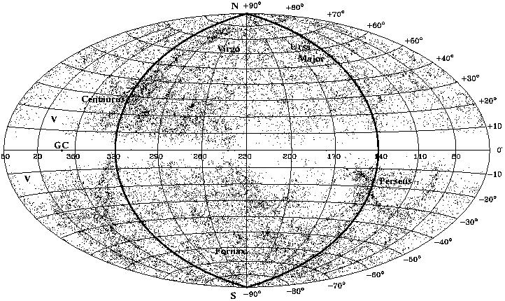
As we look out into the sky, it is quite clear that galaxies are not spread uniformly through space, but are clumped into groups and rich clusters. Figure 7.1 shows the positions on the sky of almost 15 000 bright galaxies, taken from three different catalogues compiled from optical photographs. Very few of them are seen close to the plane of the Milky Way's disk at b = 0, and this region is sometimes called the Zone of Avoidance. The term is unfair: surveys in the 21 cm line of neutral hydrogen, and in far-infrared light, show that galaxies are indeed present, but their visible light is obscured by dust in the Milky Way's disk. Dense areas on the map mark rich clusters: the Virgo cluster is close to the north Galactic pole, at b = 90°. Few galaxies are seen in the Local Void, stretching from l = 40°, b = -20° across to l = 0, b = 30°.

Figure 7.1. Positions of 14 650 bright galaxies, in Galactic longitude l and latitude b. Many lie near the supergalactic plane, approximately along the Great Circle l = 140° and l = 320° (heavy line); V marks the Local Void. Galaxies near the plane b = 0 of the Milky Way's disk are hidden by dust - T. Kolatt, O. Lahav.

The galaxy clusters themselves are not spread evenly on the sky: those within about 100 Mpc form a rough ellipsoid lying almost perpendicular to the Milky Way's disk. The Hydra-Centaurus concentration of galaxies in Figure 1.18, the Ursa Major group of Figures 5.6 and 5.8, and the Perseus cluster of Figure 6.26, all lie close to the Great Circle through Galactic longitude l = 140° and l = 320°, shown as a heavy line in Figure 7.1. The equator of the ellipsoid is the supergalactic plane; it is well-defined in the northern Galactic hemisphere (b > 0), but becomes rather scruffy in the south.

We often use supergalactic coordinates to describe the positions of nearby galaxies. The pole or Z axis of the supergalactic plane points to l = 47.4°, b = 6.3°. We take the supergalactic X direction in the Galactic plane, pointing to l = 137.3°, b = 0, while the Y axis points close to the north Galactic pole at b = 90°, so that Y 0 along the Zone of Avoidance. The supergalactic plane passes through the nearby Virgo cluster at right ascension = 12^h, declination = 12°; the Perseus cluster, at = 3^h, = 40°; and Fornax, at = 4^h, = -35°.

Figure 7.2 shows the positions of nearby elliptical galaxies, within about 20 Mpc. The distances to these objects have been found by analyzing surface brightness fluctuations. Even though the galaxies are too far away for us to distinguish individual bright stars, the number N of stars falling within any arcsecond square on the image has some random variation; so the surface brightness of any square fluctuates about some average value. The closer the galaxy, the fewer stars lie within each square, and the stronger the fluctuations between neighboring squares: when N is large, the fractional variation is proportional to 1 / N. So if we measure the surface brightness fluctuations in two galaxies where we know the relative luminosity of the bright stars that emit most of the light, we can find their relative distances.

Figure 7.2. Positions of nearby elliptical galaxies on the supergalactic X - Y plane; x shows the Milky Way. Shading indicates recession velocity Vrad - J. Tonry.

In Figure 7.2, we see that the Virgo cluster is roughly 16 Mpc away. It appears to consist of two separate pieces, which do not coincide exactly with the two velocity clumps of Section 6.5, around the galaxies M87 and M49. Here, galaxies in the northern part of the cluster, near M49, lie mainly in the nearer grouping, while those in the south near M86 are more distant; M87 lies between the two clumps. The Fornax cluster, in the south with Y < 0, is at about the same distance as Virgo. Both these clusters are seen as part of larger complexes of galaxies. Because galaxy groups contain relatively few ellipticals, they do not show up well in this figure. The Local Group is represented only by the elliptical and dwarf elliptical companions of M31, as the overlapping circles just to the right of the origin.

We can see in Figure 7.2 that galaxy clusters and groups are not very concentrated relative to their surroundings. Near the Sun, the average density of stars and gas in the Milky Way's disk corresponds to about 1 atom per cubic centimeter; this is over a million times greater than in the Universe as a whole. But in Section 6.5, we found that even in the center of a cluster like Virgo, the density of luminous galaxies is only a few thousand times more than average. Our Local Group contains only two sizable galaxies, the Milky Way and M31, plus a couple of dozen smaller ones, within a 1 Mpc radius; its density is only about ten times larger than the cosmic mean.

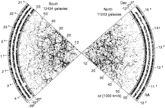
Figure 7.3 shows a `wedge diagram' with positions and measured redshifts of 24 418 galaxies in two slices across the sky: one in the south, and one in the northern sky. If we ignore peculiar velocities, Equation 1.21 tells us that the recession speed V_r cz H₀ d, where H₀ is the Hubble constant; the redshift is roughly proportional to the galaxy's distance d from our position at the apex of each wedge. So this figure gives us a somewhat distorted map of the region out to 600 h^-1 Mpc.

Figure 7.3. The Las Campanas redshift survey, covering six strips each 1.5° wide and 80° long. The northern sector is centred at b 50°, ~ l 300°, and the southern sector at b 75°, near the south Galactic pole - H. Lin, ApJ 470, 172; 1996.

The three-dimensional distribution of galaxies in Figure 7.3 has even more pronounced structure than Figure 7.1. We see dense linear features, the walls and stringlike filaments of galaxies; at their intersection are complexes of rich clusters. Between the filaments we find large regions that are almost empty of bright galaxies: these voids are typically 50h^-1 Mpc across. The galaxies appear to thin out beyond cz 40 000 km s^-1, because redshifts were measured only for objects that exceeded a fixed apparent brightness. Figure 7.4 shows that at large distances, just the rarest and most luminous systems have been included. When a solid angle on the sky is surveyed, the volume between distance d and d + d is V = d² d, which increases rapidly with d. Accordingly, we see few galaxies nearby; most of the measured objects lie near 40 000km s^-1.

Figure 7.4. Absolute R-band magnitude MR - 5 log10 h for 846 galaxies near 0h in the survey of Figure 7.3, plotted against redshift z. The arrow indicates L*, the luminosity of a typical bright galaxy; the histogram below shows numbers at each redshift. The survey included only galaxies brighter than apparent magnitude mR = 17.7 (dashed line) and fainter than mR = 15 (dotted line).}

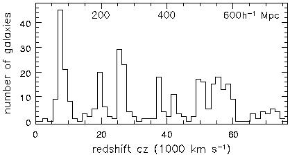
Another way to probe the large-scale distribution is to measure redshifts for galaxies within a narrow cone, but to include fainter objects. Figure 7.5 shows the redshifts of 356 galaxies near the north Galactic pole. The first peak, at redshift cz 7000 or d = 70 h^-1 Mpc, corresponds to galaxies in the Great Wall, which runs through the Coma cluster. Larger surveys show the Great Wall stretching for 100h^-1 Mpc, or a quarter of the way around the sky. Behind it, a succession of relatively empty voids alternates with more distant walls.

Figure 7.5. Distribution of redshifts for galaxies in a cone 4° x 49' across on the sky, near the north Galactic pole - see Willmer & Koo, ApJS 104, 199; 1996.

In Figures 7.3 and 7.5, the walls appear to be several times denser than the void regions. However, the use of Equation 1.21 has exaggerated their narrowness and sharpness; they would appear less pronounced if we could plot the true distances of the galaxies. The Great Wall and similar structures are still collapsing on themselves. The extra mass concentrated in a wall or filament attracts nearby galaxies in front of the structure, pulling them toward it and away from us. So the radial velocities of those objects are increased above the cosmic expansion, and we overestimate their distances, placing them further from us and closer to the wall. Conversely, galaxies behind the wall are pulled in our direction, reducing their redshifts; these systems appear nearer to us and closer to the wall than they really are. In the Great Wall, the galaxy density is only a few times higher than the local average.

By contrast, dense clusters of galaxies appear elongated in the direction toward the observer. The cores of these clusters have completed their collapse. Galaxies there are packed tightly together in space, and orbit each other with random speeds as large as 1500km s^-1, so their distances inferred from Equation 1.21 have random errors of ~ 15h^-1 Mpc. In a wedge diagram, rich clusters appear as dense `fingers', pointing toward the observer; these are especially prominent in Figure 1.18.

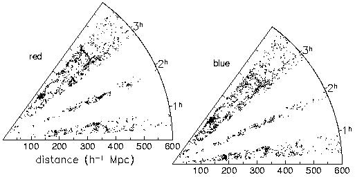
In the left panel of Figure 7.6, we clearly see a cluster near 2^h, at d = 400 h^-1 Mpc. But in the right panel, the clustering in this region is much weaker - why? The galaxies of the right panel are red in color, and their spectra show little sign of recent star formation, while in the left we see blue galaxies, with spectral lines characteristic of young massive stars and the ionized gas around them. As we saw in Section 6.5, elliptical galaxies tend to lie in the cores of rich clusters, where spiral galaxies are rare. Accordingly, the clustering of the red galaxies differs from that of the bluer systems of the right panel. The region near 0^h20^m at d =200 h^-1 Mpc is much richer in blue galaxies than red ones.

Figure 7.6. Distribution of redshifts for 2808 red galaxies (left) with spectra like elliptical galaxies, showing few young stars, and 3061 blue galaxies (right) with spectra resembling late-type spirals, in a slice of the southern sky. The elliptical-like galaxies are more strongly clustered than the spiral-like systems 2dF survey; S. Ronin, O. Lahav.