Galaxies in the Universe: An Introduction

7.1.1 Measures of galaxy clustering

One way to describe the tendency of galaxies to cluster together is the wo-point correlation function (r). If we make a random choice of two small volumes Delta V₁ and Delta V₂, and the average spatial density of galaxies is n per cubic megaparsec, then the chance of finding a galaxy in Delta V₁ is just n Delta V₁. If galaxies tend to clump together, then the probability that we then also have a galaxy in Delta V₂ will be greater when the separation r₁₂ between the two regions is small. We write the joint probability of finding a galaxy in both volumes as

(7.1)

if (r) > 0 at small r, then galaxies are clustered, while if (r) < 0, they tend to avoid each other. We generally compute (r) by estimating the galaxy distances from their redshifts, making a correction for the distortion introduced by peculiar velocities. On scales r ltapprox 50 h^-1 Mpc, it takes roughly the form

(7.2)

with gamma > 0. The probability of finding one galaxy within radius r of another is significantly larger than random when r < r₀, the correlation length. Since (r) represents the deviation from an average density, it must at some point become negative as r increases.

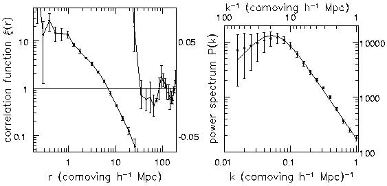
Figure 7.7 shows the two-point correlation function for galaxies of the Las Campanas survey of Figure 7.3. In the range 2 h^-1 ltapprox r 16 h^-1 Mpc where (r) is well measured, the correlation length r₀ approx 6 h^-1 Mpc and gamma approx 1.5. A rough average over many surveys gives r₀ ~ 5 h^-1 Mpc, and gamma ~ 1.8. The two-Point correlation function oscillates around zero for r gtapprox 30 h^-1 Mpc, roughly the size of the largest wall or void features; the galaxy distribution is fairly uniform on larger scales.

Figure 7.7. Left, correlation function (r) for the Las Campanas galaxy survey, at small separation (left logarithmic scale) and large (right linear scale). Vertical bars show uncertainties; redshifts were converted to distances assuming Omega ₀ = 1. Right, power spectrum P(k); the smooth curve shows a fitting function that joins smoothly to constraints from COBE at small k - H. Lin, D. Tucker.

Unfortunately, the correlation function is not very useful for describing the one-dimensional filaments or two-dimensional walls of Figure 7.3. If our volume Delta V₁ lies in one of these, the probability of finding a galaxy in Delta V₂ is high only when it also lies within the structure. Since (r) is an average over all possible placements of Delta V₂, it will not rise far above zero once the separation r exceeds the thickness of the wall or filament. We can try to overcome this by defining the three-point and four-point correlation functions, which give the joint probability of finding galaxies in each of three or four distinct volumes; but this is not very satisfactory. A good statistical method has yet to be developed to describe the strength and prevalence of walls and filaments.

The Fourier transform of (r) is the power spectrum P(k):

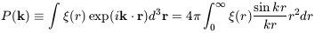
(7.3)

so that small k corresponds to a large spatial scale. Since (r) is dimensionless, P(k) has the dimensions of a volume. The function sin kr / kr is positive for |kr| < , and it oscillates with decreasing amplitude as kr becomes large; so very roughly, P(k) will have its maximum when k^-1 is close to the radius where (r) drops to zero. The right panel of Figure 7.7 shows that when k is large, we have P(k) propto k^-1.8; the power spectrum flattens and starts to decline for k^-1 gtapprox 60 h^-1 Mpc.

Problem 7.4: Prove the last equality of Equation 7.3. One method is to write the volume integral for P(k) in spherical polar coordinates r, theta , phi and set k . r = k r cos theta . Show that because (r) describes departures from the mean density, Equation 7.1 implies integ ₀ (r) r² dr = 0, and hence P(k) -> 0 as k -> 0.

Problem 7.5: Show that the power spectrum P(k) propto kⁿ corresponds to a correlation function (r) propto r^-(3+n). Hence gamma approx 1.5 implies n approx - 1.5, approximately as we see in Figure 7.7

We can write the local density at position x as a multiple of the mean level rhobar , as rho (x) = rhobar [1 + delta (x)], and let delta _R be the fractional deviation delta (x) averaged within a sphere of radius R. When we take the average < delta _R > over all such spheres, this must be zero. The dimensionless quantity < delta _R² > measures the lumpiness or non-uniformity of the galaxy distribution on this scale. We can relate < delta _R² > to k³ P(k), the dimensionless number prescribing the fluctuation in density within a volume k^-1 Mpc in radius. If clumps of galaxies with size k^-1 are placed randomly in relation to those on larger or smaller scales (the random phase hypothesis), we have

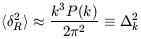
(7.4)

where k approx R^-1. We often parametrize the clustering by sigma ₈, defined as the average fluctuation on a scale R = 8 h^-1 Mpc. For the Las Campanas survey, sigma ₈ approx 1. Since P(k) declines more slowly than k^-3 at high wavenumbers, Delta _k² increases with k. The smaller the region we consider, the greater the probability of finding a very high density of galaxies. Cosmological models for the development of structure can predict P(k), for comparison with observations; we return to this topic in Section 7.4.

Problem 7.6: The quantity < Delta _k² >^1/2 gives the expected fractional deviation | delta (x)| from the mean density in an overdense or diffuse region of size 1 / k. Use Equation 3.9, Poisson's equation, to show that these lumps and voids cause fluctuations Delta phi _k in the gravitational potential, where k² | Delta phi _k| ~ 4 G rhoba r < Delta _k² >^1/2. Show that when P(k) propto k, the Harrison-Zel'dovich spectrum, the amplitude of Delta phi _k does not depend on k: the potential is equally `rippled' on all spatial scales.

In this section we have seen that the present-day distribution of galaxies is very lumpy and inhomogeneous on scales up to 100 h^-1 Mpc. But measurements of the cosmic background radiation show that its temperature is the same in all parts of the sky to within a few parts in 100 000. Thus at the time of recombination, when the pregalactic gas became neutral and transparent, matter and radiation were very smoothly distributed. How could our present highly structured Universe of galaxies have arisen from such uniform beginnings? To understand what might have happened, we must begin by looking at how the Universe expanded following the Big Bang, and how concentrations of galaxies could form within it.