


1. Radioactive decay
For my first trick, let's assume that you have a radioactive sample in
a physics laboratory, and with your trusty Geiger counter you want to
determine the amount of some short-lived radioactive isotope present
in the sample. Observing over a total span of 30 minutes, you detect
the numbers of radioactive events which I have listed in
Table 1-1.
How much radioactive isotope was present at time t = 0, when the
sample first came out of the accelerator where it had been bombarded
with high-energy particles? The first thing that I want you to notice
is that the raw data are simple number counts, and it is reasonable to
expect that the uncertainty in any of these numbers is determined by
Poisson statistics. (In fact, when I made up these data I added
random Poisson noise.) Thus, we should have an excellent handle on
what the observational errors ought to be. Since the raw number counts
were integrated over different lengths of time, I have converted them
to counting rates Ri by dividing the observed number
counts Ni by
 t;
the standard errors of these counting rates are also obtained by
dividing the standard errors of the number counts by
t. I suggest
that we use the midpoint of each observation as the independent
variable. This is not really the right thing to do (see if you can
figure out why), but it is close enough for government work. Suppose
we believe that our radioactive sample should consist of a pure
isotope with a known half-life of seven minutes. As you know, apart
from the random Poisson noise, radioactive decay follows an
exponential function of time:
t;
the standard errors of these counting rates are also obtained by
dividing the standard errors of the number counts by
t. I suggest
that we use the midpoint of each observation as the independent
variable. This is not really the right thing to do (see if you can
figure out why), but it is close enough for government work. Suppose
we believe that our radioactive sample should consist of a pure
isotope with a known half-life of seven minutes. As you know, apart
from the random Poisson noise, radioactive decay follows an
exponential function of time:
where the parameter A simply represents the rate of decays at time t =
0 (which, of course, is proportional to the isotope's abundance, which
is what we want to know), and
then this is in exactly the same form as a problem we've seen before,
that of fitting the slope of a straight line to data while forcing
that line to pass through the origin. (In this case, the origin x = 0
occurs at time t =
where I have used
I have illustrated this fit in Fig. 1-2, both
as a function of the
linearized coordinate x (upper), and as a function of the actual time
t = -ln(x) /
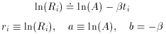
Well, then, suppose it's a pure isotope with some other, unknown,
half-life? The equation describing this situation is, of course,
Ri
then we get
an equation that is linear in the two new unknowns, a and
b. The only
tricky thing that we have to watch out for is that the standard error
of each data point must also be properly transformed to the new
variables:
(More on this propagation of error stuff next time. Watch for it. For
now, be aware that this conversion is not mathematically perfect, in
the sense that if Ri is distributed as a Gaussian
random variable, ri
will not be. In fact, even Ri is not distributed as a
Gaussian
variable, but rather as a Poisson variable, so we shouldn't really be
doing least squares at all. However, as long as
and
Fig. 1-3 contains two plots illustrating this
fit, which obviously
looks much better than the previous one, but is still not perfect. The
mean error of unit weight is 2.01, or
I won't keep you in suspense any longer. I made up these data assuming
that the sample was actually a mixture of three different isotopes
with half-lives of 4, 7, and 23 minutes. Once you know this, you can
now use linear least squares to calculate how much each of these
isotopes contributes to the overall radioactivity. Once again, you
have to make a certain substitution of variables to make it perfectly
clear that this is in fact a problem in linear least squares, but that
is not a difficulty:
Let xj, i =
exp(-
Does this look the least little bit familiar? Once you have turned the
crank on the machinery that I set up before, you get
In other words, once you get the model right (I told you that there
were three components, and I even gave you the half-lives) the mean
error of unit weight comes out to a value near one, just as it
should. You might like to compare these results for the number of
decays due to each component to the values which I put in, to generate
these data: I used A1 = 214.0, A2 =
569.0, and A3 = 321.0. As you can
see, the agreement between the input and output values for the three
unknowns do not show perfect agreement - after all, I did generate
reasonable, random, Poisson errors for the "observations." Still, the
agreement is consistent with the error bars. How did I get these error
bars? I'll tell you next time.
There is one other thing that is interesting to note. The error bars
on
One very last point. Suppose I told you that there were three
components, but I didn't give you the half-lives: could you still
solve for six unknowns, three abundances and three half-lives? Ah! Now
there's a problem that can't be done with linear least squares. More
about that next time.
 is the natural
logarithm of 2 divided
by the half-life. How can we use least squares to determine the value
of A, given the assumption that the half-life is seven minutes? Well,
it's perfectly easy. All you have to do is recognize is that if you
make the substitution x =
e-t, so
is the natural
logarithm of 2 divided
by the half-life. How can we use least squares to determine the value
of A, given the assumption that the half-life is seven minutes? Well,
it's perfectly easy. All you have to do is recognize is that if you
make the substitution x =
e-t, so

 - we
are requiring our solution to give zero
abundance for the radioactive isotope after an infinite amount of time
has passed. This is eminently reasonable.) We all remember the formula
for that problem, and here it is: the best fit for the number of
decays per unit time at t = 0 is
- we
are requiring our solution to give zero
abundance for the radioactive isotope after an infinite amount of time
has passed. This is eminently reasonable.) We all remember the formula
for that problem, and here it is: the best fit for the number of
decays per unit time at t = 0 is
time N
 N
N R

(min) =N /
t
= N /
t
0.0-1.0 1032 32.1 1032 32.1
1.0-2.0 917 30.3 917 30.3
2.0-4.0 1643 40.5 822 20.3
4.0-6.0 1416 37.6 708 18.8
6.0-8.0 1243 35.3 622 17.6
8.0-12.0 1865 43.2 466 10.8
12.0-16.0 1513 38.9 378 9.7
16.0-20.0 1210 34.8 302 8.7
20.0-24.0 967 31.1 242 7.8
24.0-30.0 1074 32.8 179 5.5
(lower). As you
can see, the "best" fit is a very poor
one, a conclusion which is reinforced by the mean error of unit
weight: if you compute the weighted mean square residual (remember, I
have used s = 1), you find m.e.1 = 8.79. (Try it!) In other words, the
residuals are almost nine times larger, on average, than they should
be. A chi-squared test will tell you that you should never see scatter
this large with standard errors like these
( 2 = 695 for 9 degrees of
freedom). These are simple Poisson errors! We can't have got them that
far wrong! The problem must be with our assumptions: our prediction
that the radioactive sample should have a half-life of seven minutes
was wrong.
2 = 695 for 9 degrees of
freedom). These are simple Poisson errors! We can't have got them that
far wrong! The problem must be with our assumptions: our prediction
that the radioactive sample should have a half-life of seven minutes
was wrong.
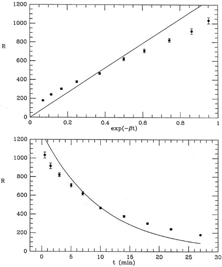
Figure 1-2
 Ae-ti, which now has two unknown quantities,
A and . Now
you can't
solve this equation by least squares, at least not with the techniques
that I've just shown you, because the equation is not linear in the
unknown parameters, A and
. However, you can
still make linear least
squares work here by yet another change of variables. If we take the
logarithm of both sides of this equation, and make three simple
substitutions,
Ae-ti, which now has two unknown quantities,
A and . Now
you can't
solve this equation by least squares, at least not with the techniques
that I've just shown you, because the equation is not linear in the
unknown parameters, A and
. However, you can
still make linear least
squares work here by yet another change of variables. If we take the
logarithm of both sides of this equation, and make three simple
substitutions,

 (R) is small compared
to R, both these subtleties can be swept under the rug - they will
introduce systematic errors many orders of magnitude smaller than
those inherent to our small data set. Just so you know.) Now we can
solve for the best estimates of a and b using the standard linear
least squares that we have seen before. When we do this we get
(R) is small compared
to R, both these subtleties can be swept under the rug - they will
introduce systematic errors many orders of magnitude smaller than
those inherent to our small data set. Just so you know.) Now we can
solve for the best estimates of a and b using the standard linear
least squares that we have seen before. When we do this we get
 2 = 32.3 for 8 degrees of
freedom. Your handy table of reduced
2 values tells you that this is
still very unlikely to be the correct answer: the probability of
getting this value of 2
if all the assumptions are correct is only about one in 104.
2 = 32.3 for 8 degrees of
freedom. Your handy table of reduced
2 values tells you that this is
still very unlikely to be the correct answer: the probability of
getting this value of 2
if all the assumptions are correct is only about one in 104.
Figure 1-3
 j
ti) and you have
j
ti) and you have
 1 and
2 are much larger than
the error bars on 3.
There's a very
simple explanation for this: the half-lives of 4 and 7 minutes are
just too similar, given the spacing of the data points. If you look at
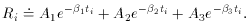
the two rapidly decaying curves in Fig. 1-4,
you can see that their
shapes are very similar, and the coefficient of each is most strongly
constrained by the innermost three or four data points. The shape of
the slow-decaying curve is quite different, and the last three or four
data points are more strongly determined by it than by the other two
curves put together. In other words, the available observations do
not strongly distinguish between the 4- and 7-minute half-lives: you
could decrease the inferred fraction of one component, increase the
fraction of the other, and not make a big difference in the quality of
the fit. That is why the uncertainties in the proportions of the first
two components are large. On the other hand, the abundance of the last
component is well determined by the last few data points; that is why
its uncertainty is small. One often hears the complaint that
least-squares problems are ill-determined. That is not true of a
well-designed experiment, in general. This is one of those rare,
unfortunate cases, where the experiment is ill-designed, at least from
the point of view of distinguishing between the first two radioactive
components. Too bad the experimenter didn't start taking data 10 or 15
minutes earlier (while the sample was still in the particle
accelerator?). Then the difference between the 4- and 7-minute
half-lives would have been obvious.
1 and
2 are much larger than
the error bars on 3.
There's a very
simple explanation for this: the half-lives of 4 and 7 minutes are
just too similar, given the spacing of the data points. If you look at
the two rapidly decaying curves in Fig. 1-4,
you can see that their
shapes are very similar, and the coefficient of each is most strongly
constrained by the innermost three or four data points. The shape of
the slow-decaying curve is quite different, and the last three or four
data points are more strongly determined by it than by the other two
curves put together. In other words, the available observations do
not strongly distinguish between the 4- and 7-minute half-lives: you
could decrease the inferred fraction of one component, increase the
fraction of the other, and not make a big difference in the quality of
the fit. That is why the uncertainties in the proportions of the first
two components are large. On the other hand, the abundance of the last
component is well determined by the last few data points; that is why
its uncertainty is small. One often hears the complaint that
least-squares problems are ill-determined. That is not true of a
well-designed experiment, in general. This is one of those rare,
unfortunate cases, where the experiment is ill-designed, at least from
the point of view of distinguishing between the first two radioactive
components. Too bad the experimenter didn't start taking data 10 or 15
minutes earlier (while the sample was still in the particle
accelerator?). Then the difference between the 4- and 7-minute
half-lives would have been obvious.
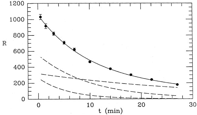
Figure 1-4