


2. Parallel lines
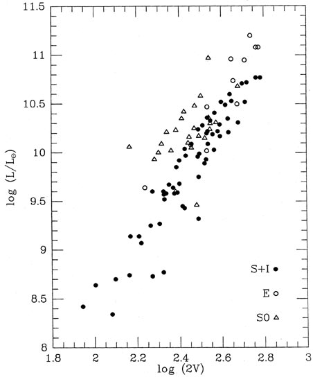
The data illustrated in Fig. 1-5 were very kindly lent to me by Dr. Michael Pierce. They represent the luminosities of three different classes of galaxies in the Virgo cluster - (1) spirals and irregulars, (2) ellipticals, and (3) lenticulars (S0's) - plotted against some measure of the internal velocities: for the spirals and irregulars, it is twice the Vmax obtained from the integrated 21-cm line profile, while for the ellipticals and lenticulars, it is twice the central velocity dispersion obtained from the stellar absorption-line profiles. For the purposes of this example, let us assume that you have some astrophysical theory that tells you that these three relationships between luminosity and internal velocity should all be perfectly linear (the classical Tully-Fisher and Faber-Jackson relationships) with exactly the same - though unknown - slope, and three different zero-points. What is the best way to determine the unknown slope and the three unknown zero-points from these data? The most obvious way to approach the problem (and the way which, I think, most astronomers would try first) is simply to separate the three data sets, and fit straight lines to them independently. Then you'd average together the three slopes that you'd gotten, and assuming that mean slope to be correct, you'd go back and redetermine the three zero-points. That isn't really the best way to go, however. In particular, notice that the ellipticals span a much smaller range of luminosity and velocity than the spirals. The estimated slope that you'd get from the spiral-galaxy data should be of much higher quality than the slope from the ellipticals, and you'd have to be very careful to take this into account when you determined the mean slope. Furthermore, in some sense you're using these data to estimate six quantities (three slopes and three zero-points) when all you really want is four (one slope and three zero-points). There's a much more direct - and statistically more sensible - path to the specific results that you really want.
|
| Figure 1-5 |
The trick is to realize that the ti in the equation
don't have to be continuous variables, they can be anything that you
can assign a numerical value to. In particular, you can let some of
them be Kronecker
Now crank these data through the machinery:
(assuming all galaxies have equal weight, even if they don't have
equal mass). From

 's:
's:
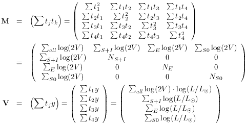
 =
M-1V you get
=
M-1V you get
 1 = the one best
slope that fits all the data sets taken together,
2 = the zero-point for
the spirals and irregulars,
3 = the zero-point for
the ellipticals, and 4 = the
zero-point for the lenticulars. (All in one fell swoop.) The bundle of
three best-fitting parallel lines is illustrated in
Fig. 1-6.
1 = the one best
slope that fits all the data sets taken together,
2 = the zero-point for
the spirals and irregulars,
3 = the zero-point for
the ellipticals, and 4 = the
zero-point for the lenticulars. (All in one fell swoop.) The bundle of
three best-fitting parallel lines is illustrated in
Fig. 1-6.

Figure 1-6