LECTURE 2

PARAMETER ERROR ESTIMATES AND NONLINEAR LEAST SQUARES

A. Parameter error estimates

In my previous lecture, I promised that I would explain how to derive standard-error estimates for the derived fitting parameters. To provide some background for the subject, let's take a look at how errors propagate. Let's say you have some continuous function f of a variable x, and that any specific value of that x is subject to random errors. To first order the standard error of the f corresponding to that x is given by

If f is a linear function of x then this equation is exact; if the function is non-linear then this relationship is only good, as I said, to first order. Now if f is a function of many independent variables x, then to obtain the overall standard error of f you have to add the squares of the individual contributions, like this:

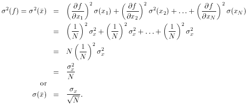
Just for practice, let's apply this equation to a very simple linear function. Let f be the mean of N independent determinations of some quantity x, where each x measurement is subject to a constant standard error, _x. Then f = (x₁ + x₂ + . . . x_N) / N, and the square of the random error of f is given by

Thus, we finally arrive at something you knew all along, namely when you take the average of N independent measurements of some quantity, the standard error of the mean decreases as the square root of N.

Now let's look at the case where the standard errors of the individual x measurements are not the same, so we want to take a weighted mean of the x measurements. The weights are given, as usual, by the inverse squares of the standard errors:

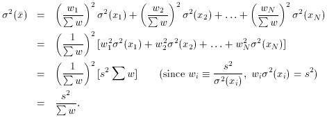
When we now propagate the errors through this equation, we see

So we conclude that

Conversely, we can also say

In other words, the weight of the weighted mean is equal to the total weight of the individual observations - an easy fact to remember.

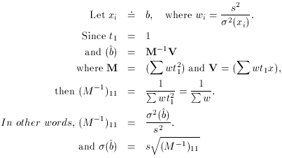
So why did I bother to go through all that? Well, let's look at the problem again, but this time using the least-squares formalism presented in the last lecture:

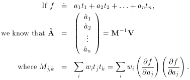
I'm not going to give you a formal proof - they can be found in more advanced texts on maximum-likelihood techniques - but the same sort of conclusion can be drawn with greater generality:

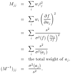
The diagonal elements of M are

So...

As a footnote: the off-diagonal elements of M^-1 give the correlation coefficients, r_{k, k} between the parameters: