


1. Fitting a model profile to a star image
|
| Figure 2-1 |
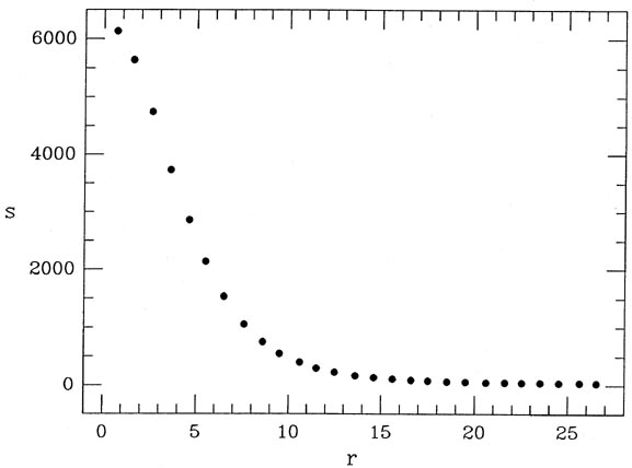
In Fig. 2-1 I illustrate an observed radial intensity profile for a star. To obtain this profile I took the actual digital data for an isolated star in a CCD image which I happened to have, estimated the position of the star's centroid by eye, and obtained the average intensity within the star image as a function of the radial distance from the center by averaging the observed pixel values in narrow, concentric annuli. Now, it has been known for a long time that the so-called "Moffat" function is a very good representation of the radial profile of a star image (Moffat 1969; Buonanno, et al. 1983). In its simplest useful form, the Moffat function is
where S stands for the Specific intensity (or, if you prefer, the
Surface brightness) at some point located a radial distance r (=
sqrt[(x - x0)2 + (y -
y0)2]) from the center of the stellar
image. As you can see,
besides the independent variable r, the Moffat function also involves
four unknown parameters, which must be determined empirically: I
denote them B, which is the Background diffuse sky
brightness caused
by emission from Earth's atmosphere, zodiacal light, unresolved
background galaxies, and so on (i.e., B =
limr->
Of course, in real life we can't integrate a stellar profile to
infinity; we can observe it only out to
For the sake of pursuing this first example, let us assume that the
value of
(Remember, for the time being we're assuming that
Similarly,
and
The magical difference between this problem and the linear
least-squares problems we looked at in the previous lecture is this:
whereas before, when we took
the derivatives ð
The way out is to use one of the favorite tools of mathematical
physicists (and statisticians like it, too!): the method of successive
approximation. That is, we guess at approximate solutions for our
three unknowns, C, B, and R; I will call these
guesses C0, B0, and
R0. If we write the final, least-squares solution that
we want so
badly as S(r;
which leads to the set of fitting equations
or, equivalently,
We may recognize that this equation is of the same form as
where
and
We already know how to solve these linear equations for the three
unknown parameters
and try again. These new equations can now be solved for fresh values of
A GENERAL METHODOLOGY FOR NONLINEAR LEAST SQUARES
Step 1.
Write down your analytic equation, and derive its first derivative with
respect to each of
the unknown fitting parameters. In the example above,
Step 2.
By any means available, guesstimate approximate values for the fitting
parameters. For
instance, in the example above you might take the largest observed value
of si as your
initial guess for C, and sN as your initial
guess at B. These guesses don't have to be "best"
values - that's why we're doing the least squares. They just have to be
vaguely all right (except sometimes).
Step 3.
For each data point, calculate the error of the initial model, and use
these residuals to solve
for corrections to the parameter estimates by ordinary linear least
squares. In the example
above, this step is represented by the equation
Step 4.
Add the parameter corrections which you have just computed to your
initial guesses at the parameter values, to obtain improved parameter values.
Step 5.
Examine the parameter corrections which you computed in Step 3. How big
are they? If
any or all of them are larger than you would like, go back and do Steps
3 and 4 again. Keep
doing Steps 3, 4, and 5 until all parameter corrections are negligibly
small. When this is
accomplished, you have achieved your desired least-squares solution!
Step 5 (alternate).
Using the current set of parameter estimates, calculate the m.e.1 of
your data points with
respect to the current model. In the notation of the example above, this
would be
Repeat Steps 3, 4, and 5 as long as the m.e.1 continues to get
significantly smaller. When the
root-mean squar e residual no longer decreases with additional
iterations, you have achieved your desired least-squares solution!
Whether you choose to adopt Step 5 or Step 5 (alternate) may depend upon
why you
want to solve the least-squares problem in the first place. If you are
actually interested
in the best numerical values for the fitting parameters, you will want
to use Step 5. For
instance, if you are fitting the model profile to the star image because
you want to know
how bright the star is, what you want is accurate values for C and
R. Another example is
the radioactive decay experiment from my last lecture, where you really
wanted to know
the actual abundances of each of the isotopes: if for some reason you
found yourself doing
iterated least squares (cf. Lecture 3) you
would keep iterating until you got the parameter
values as accurately as you could; you would adopt Step 5 as your
convergence criterion.
However, suppose you wanted to model a stellar surface-brightness
distribution simply in
order to interpolate the star's intensity profile to some radius between
two of your ri values?
In this case you don't really care what C and R are, you
just want to know that the model
represents the data to the required level of precision. Therefore you
might adopt Step 5
(alternate). Similarly, in the problem where we transformed the
coordinate systems of CCD
frames yesterday: maybe you aren't interested in the actual values of
the translation, scale,
and rotation constants, you just want to be sure that the
transformations are good to, say,
0.1 pixel for the average star; if you had to iterate the solution for
some reason, you would
stop iterating when and if the mean error of unit weight dropped
significantly below this value.
I guess this is a good time to ramble on philosophically about some of
the subtleties
involved here. Which brings me to my first statement of a theme which
will recur throughout
the rest of these lectures, to wit: computers may be awfully smart, but
computers are awfully
stupid! The computers available today, at least, may be really good at
arithmetic but they
aren't yet much for common sense. One of the best examples of this is
they don't know
when to quit. If you tell the computer to go and compute sums and invert
matrices until
As I said above, there are various ways this can be done in our profile-fitting
problem, and I'd like you to think about some of them for a moment: you
might tell
the computer to quit when the size of the correction to the central
surface brightness drops
to |
Now, back to the example. Figs. 2-2 and
2-3 represent a nonlinear
least-squares fit of
a Lorentz function (a Moffat function with
Fig. 2-3 shows the raw data as points, the
"initial guess" at the solution as the dashed
curve which peaks near 4000, the improved solution after a single
iteration as the other
dashed curve, and the final solution as the solid curve. I think you can
see that, even with
pretty horrible initial guesses at the solution, after one or two hops
to get itself into the
right ballpark, the solution converges like a bat out of . . ., the
solution converges pretty
quickly. Still, real afficionados would not be satisfied with this fit
for two reasons: first,
if you look carefully at Fig. 2-3 you'll see
that the data points tend to fall consistently
below the best solution for 8
What shall we do about this? One obvious solution is to admit that we
were pretty foolish to assume that
Well, I always have to go back to the CRC Tables for this one, but
is what we need to work out
Let a -> 1 + r2 / R2,
u -> -
So now we've got it knocked. We just perform our same old linearized
nonlinear least-squares
solution for four unknowns rather than three. The results of this
exercise are shown
in Fig. 2-4. As you can see, by merely solving
for
Just for fun, I ran the four-parameter fit again with a different set of
starting guesses;
the printout from this reduction is shown as
Fig. 2-5. Oops. This is yet
another example
of the fundamental stupidity of the computer. I told the heap of dirty
silicon to evaluate
some algebraic derivatives, compute some sums, invert and multiply some
matrices, and
add the resulting numbers to the original numbers, and that's what it
did. It didn't notice
- or care - that the results were garbage; if I didn't warn it to watch
out for trouble it
sure wasn't going to notice trouble on its own. The problem here is that
sometimes the
first-order Taylor expansion is not quite good enough. Certainly, given
any set of fitting
parameters, you can compute the value of
The way around the problem is for the human being to anticipate that this might
happen and forewarn the computer to watch out for it. Stepping back from
the problem
once again, we remind ourselves that the first derivatives of
I figured that C and B were well enough constrained by the
data that, if
R and
This is a good place to stress that "clamps" or any other arbitrary
scheme for coming
up with parameter corrections do not mean that you are fudging the data
in any way, shape,
or form. The heart and soul of the method of least squares consist in
finding the minimum of
1 By the same sort of change of variables
that we did in the
radioactive decay examples: let the known quantity be
si
2 This is a great place for minus signs
to trip you up. The left-hand side of the fitting
equation is the negative of
 S(r),
as you can
easily confirm); C, representing the star's Central
surface brightness
above the local background (i.e., C = S(r =
0) - B, ¿no es verdad?);
then there is R, which is a sort of characteristic Radius
of the star
image, determined by such broadening mechanisms as seeing, and guiding
errors; and finally, there is
S(r),
as you can
easily confirm); C, representing the star's Central
surface brightness
above the local background (i.e., C = S(r =
0) - B, ¿no es verdad?);
then there is R, which is a sort of characteristic Radius
of the star
image, determined by such broadening mechanisms as seeing, and guiding
errors; and finally, there is
 , which describes
the asymptotic
power-law slope of the wings of the image at large radial distances
from the center (that is, for large r, S(r) - B ->
C . (r2 /
R2)-). In
particular, if =
1, then the stellar profile is a Lorentz function,
and R is the half-width at half maximum, since in this case
S(R) - B = C / 2. (However, real star images cannot be
perfect Lorentz profiles since
, which describes
the asymptotic
power-law slope of the wings of the image at large radial distances
from the center (that is, for large r, S(r) - B ->
C . (r2 /
R2)-). In
particular, if =
1, then the stellar profile is a Lorentz function,
and R is the half-width at half maximum, since in this case
S(R) - B = C / 2. (However, real star images cannot be
perfect Lorentz profiles since
 radians if the star is at
the zenith! However, the Lorentz profile still has an unreasonable
amount of flux out in the wings.)
is
known. If we also assume that R is known, then the
problem is linear in the unknowns C and
B (1) so we
know how to do the
least-squares solution. But let's take it to the next degree of
difficulty, and assume that we want to solve for C, B, and
the seeing
parameter R all at once. How shall we do this? Well, we have to go
back to the basics. The whole thing about "least squares" is you want
to minimize the sum of the squares of the fitting residuals - that's
how you get the maximum-likelihood answer, and that hasn't
changed. Where does it occur that
radians if the star is at
the zenith! However, the Lorentz profile still has an unreasonable
amount of flux out in the wings.)
is
known. If we also assume that R is known, then the
problem is linear in the unknowns C and
B (1) so we
know how to do the
least-squares solution. But let's take it to the next degree of
difficulty, and assume that we want to solve for C, B, and
the seeing
parameter R all at once. How shall we do this? Well, we have to go
back to the basics. The whole thing about "least squares" is you want
to minimize the sum of the squares of the fitting residuals - that's
how you get the maximum-likelihood answer, and that hasn't
changed. Where does it occur that
 2 =
2 =

 2 minimized?
Why, at the point where the first derivative of
2 with respect to every one of
the fitting parameters is zero, simultaneously. Let's do it.
2 minimized?
Why, at the point where the first derivative of
2 with respect to every one of
the fitting parameters is zero, simultaneously. Let's do it.
 is known.)
 /
ða did not contain any unknown fitting parameters, a,
- they depended only upon known quantities, t. Obviously, that's
because those equations were linear in the fitting parameters, a. That
meant that we were able to pull the constant (but unknown) fitting
parameters from the 's out
of the summations. The summations that
were left then included only known quantities; they could be computed;
and the resulting system of equations - all of which were linear in
the unknown parameters - could be solved for the a's. In our current
problem, the ð /
ða's do contain a's; the unknowns can't be taken out of
the summations; the summations can't be evaluated; and we can't solve
for the parameters until after we know them.
/
ða did not contain any unknown fitting parameters, a,
- they depended only upon known quantities, t. Obviously, that's
because those equations were linear in the fitting parameters, a. That
meant that we were able to pull the constant (but unknown) fitting
parameters from the 's out
of the summations. The summations that
were left then included only known quantities; they could be computed;
and the resulting system of equations - all of which were linear in
the unknown parameters - could be solved for the a's. In our current
problem, the ð /
ða's do contain a's; the unknowns can't be taken out of
the summations; the summations can't be evaluated; and we can't solve
for the parameters until after we know them.
 ,
,
 ,
,
 ), we can approximate this by a
Taylor expansion evaluated with our initial guesses:
), we can approximate this by a
Taylor expansion evaluated with our initial guesses:

 C,
B, and
R. When we crank up the
old machinery we can compute the improved
parameter values C1 = C0 +
C, B1
= B0 + B,
and R1 = R0 +
R.
(2) Unfortunately,
because our first-order Taylor expansion is only approximate, we can be
reasonably certain
that the new values C1, B1, and
R1 will not be exactly equal to the best
values ,
, and
- which is why I dropped the "^"
notation and used the subscript1 instead - and
they probably won't even be "good enough for all practical purposes."
Nevertheless, they
should be better estimates than C0,
B0, and R0 were. So, we just plug
them back into the equations,
C,
B, and
R. When we crank up the
old machinery we can compute the improved
parameter values C1 = C0 +
C, B1
= B0 + B,
and R1 = R0 +
R.
(2) Unfortunately,
because our first-order Taylor expansion is only approximate, we can be
reasonably certain
that the new values C1, B1, and
R1 will not be exactly equal to the best
values ,
, and
- which is why I dropped the "^"
notation and used the subscript1 instead - and
they probably won't even be "good enough for all practical purposes."
Nevertheless, they
should be better estimates than C0,
B0, and R0 were. So, we just plug
them back into the equations,
 C,
B, and
R
(which should mostly be smaller than the previous ones), and we may take
C2 = C1 +
C,
B2 = B1 +
B, and
R2 = R1 +
R as still better
estimates of the desired fitting parameters.
This whole process may be repeated as many times as necessary. Of
course, as C,
B,
and R become smaller and
smaller, the Taylor expansion becomes better and better. The
solution should quickly converge, and when
C,
B, and
R have all
become negligibly
small we have found the least-squares solution to our problem. This
leads me to . . .
C,
B, and
R
(which should mostly be smaller than the previous ones), and we may take
C2 = C1 +
C,
B2 = B1 +
B, and
R2 = R1 +
R as still better
estimates of the desired fitting parameters.
This whole process may be repeated as many times as necessary. Of
course, as C,
B,
and R become smaller and
smaller, the Taylor expansion becomes better and better. The
solution should quickly converge, and when
C,
B, and
R have all
become negligibly
small we have found the least-squares solution to our problem. This
leads me to . . .
 C,
B, and
R go to zero, the
computer will keep on going forever or until the next
power failure, whichever comes first. Because of truncation error,
ð2 / ðC
probably will
never go identically to zero: after an infinite amount of iterating,
your current best value
of C will give still you a finite value for
C, but try to improve your
estimate of C by
one quantum in the least significant bit, and you'll get another finite
correction C of
the opposite sign. It's time for the astronomer/programmer to step in
and impose a little
common sense. When you write the program, you must decide ahead of time
just how good
you need your answer to be, and tell the computer that it is allowed to
quit when it gets there.
C| < 0.001 electrons
per pixel; alternatively, since the likelihood
is that you really want
C in order to compute the star's magnitude by some formula like
magnitude = constant - 2.5 log C,
you could tell the computer to quit when
|C| < 0.001C -
when an iteration
changes the star's brightness by less than a millimagnitude. Of course,
for faint stars,
you're never going to get an answer good to a millimagnitude anyway,
just because of the
noise, so maybe you'll tell the computer to quit when
|C| < 0.1
C,
B, and
R go to zero, the
computer will keep on going forever or until the next
power failure, whichever comes first. Because of truncation error,
ð2 / ðC
probably will
never go identically to zero: after an infinite amount of iterating,
your current best value
of C will give still you a finite value for
C, but try to improve your
estimate of C by
one quantum in the least significant bit, and you'll get another finite
correction C of
the opposite sign. It's time for the astronomer/programmer to step in
and impose a little
common sense. When you write the program, you must decide ahead of time
just how good
you need your answer to be, and tell the computer that it is allowed to
quit when it gets there.
C| < 0.001 electrons
per pixel; alternatively, since the likelihood
is that you really want
C in order to compute the star's magnitude by some formula like
magnitude = constant - 2.5 log C,
you could tell the computer to quit when
|C| < 0.001C -
when an iteration
changes the star's brightness by less than a millimagnitude. Of course,
for faint stars,
you're never going to get an answer good to a millimagnitude anyway,
just because of the
noise, so maybe you'll tell the computer to quit when
|C| < 0.1
 (C),
where (C)
can be computed by the method I gave you at the beginning of this
lecture. In this case
you're telling the computer to quit as soon as the correction becomes
much smaller than
the uncertainty of the correction = the uncertainty of the result. In
other cases it may
be most convenient simply to stop iterating when the m.e.1 stops
decreasing by, say, a
part in a thousand. Every situation is a little bit different, and
that's why I mostly write
my nonlinear least-squares programs from scratch every time I need to
solve a different
sort of problem. This is one of the areas where practical mathematics
becomes a creative
endeavor, where it borders on the artistic as well as the
scientific. You need to be able to
step back from the problem, see what its truly important aspects are,
and explain it to a dumb machine.
(C),
where (C)
can be computed by the method I gave you at the beginning of this
lecture. In this case
you're telling the computer to quit as soon as the correction becomes
much smaller than
the uncertainty of the correction = the uncertainty of the result. In
other cases it may
be most convenient simply to stop iterating when the m.e.1 stops
decreasing by, say, a
part in a thousand. Every situation is a little bit different, and
that's why I mostly write
my nonlinear least-squares programs from scratch every time I need to
solve a different
sort of problem. This is one of the areas where practical mathematics
becomes a creative
endeavor, where it borders on the artistic as well as the
scientific. You need to be able to
step back from the problem, see what its truly important aspects are,
and explain it to a dumb machine.
 1) to the observed
profile data illustrated
in Fig. 2-1.
Fig. 2-2 is a photocopy of my actual computer printout
documenting the
convergence of the fit. I told the computer that I wanted to solve for
three unknowns (C,
B, and R), and I then provided it with starting guesses
for the four parameters of the Moffat
function; of course,
was to be held
fixed at the value specified (
1), while the other three
were destined to be improved by the nonlinear least-squares solution. My
initial guesses
for C, B, and R were 4000, 0, and 5, respectively,
and the computer took it from there.
Succeeding pairs of lines show (upper) the current working estimates of
the three fitting
parameters C, B, and R, and (lower) the corrections
C,
B, and
R
derived from those
parameters. The last number on the upper line of each pair is the value
of the m.e.1 derived
from the differences between the data and the current model. (For this
experiment I gave
every data point unit weight; the m.e.1 therefore represents an estimate
of the r.m.s. error
of each raw datum = the brightness in a particular annulus. This isn't
what I'd do if I were
really serious; in actuality the weight should reflect the total readout
noise and the Poisson
noise in each annulus, but this is just for show so wotthehell,
wotthehell.) The last two rows
of numbers - under where it says "Converged" - represent the final
derived parameter
values and their uncertainties, calculated as described at the beginning
of this lecture. I
arbitrarily imposed a convergence criterion of 0.001 electrons per pixel
in the value of C.
As you can see, this was undoubtedly too strict since the computer could
have stopped
working several iterations sooner without producing significantly poorer
answers, whether by the milllmagnitude criterion, by
|C| <<
(C), or by the leveling-off of
2.
1) to the observed
profile data illustrated
in Fig. 2-1.
Fig. 2-2 is a photocopy of my actual computer printout
documenting the
convergence of the fit. I told the computer that I wanted to solve for
three unknowns (C,
B, and R), and I then provided it with starting guesses
for the four parameters of the Moffat
function; of course,
was to be held
fixed at the value specified (
1), while the other three
were destined to be improved by the nonlinear least-squares solution. My
initial guesses
for C, B, and R were 4000, 0, and 5, respectively,
and the computer took it from there.
Succeeding pairs of lines show (upper) the current working estimates of
the three fitting
parameters C, B, and R, and (lower) the corrections
C,
B, and
R
derived from those
parameters. The last number on the upper line of each pair is the value
of the m.e.1 derived
from the differences between the data and the current model. (For this
experiment I gave
every data point unit weight; the m.e.1 therefore represents an estimate
of the r.m.s. error
of each raw datum = the brightness in a particular annulus. This isn't
what I'd do if I were
really serious; in actuality the weight should reflect the total readout
noise and the Poisson
noise in each annulus, but this is just for show so wotthehell,
wotthehell.) The last two rows
of numbers - under where it says "Converged" - represent the final
derived parameter
values and their uncertainties, calculated as described at the beginning
of this lecture. I
arbitrarily imposed a convergence criterion of 0.001 electrons per pixel
in the value of C.
As you can see, this was undoubtedly too strict since the computer could
have stopped
working several iterations sooner without producing significantly poorer
answers, whether by the milllmagnitude criterion, by
|C| <<
(C), or by the leveling-off of
2.
Enter number of terms

3

Enter starting guesses for C, B, R, and beta

4000  0   5   1

      C	         B         R	   m.e.1

  4000.000      0.000    5.000      775.
  2757.100   -214.882   -1.947

  6757.100   -214.882    3.053      456.
  -208.755    -47.599    1.050

  6548.345   -262.481    4.104      164.
   268.906    -15.772   -0.065

  6817.251   -278.253    4.039      147.
    -3.557     -2.115    0.011

  6813.694   -280.368    4.050      147.
     0.725      0.349   -0.002

  6814.419   -280.019    4.049      147.
    -0.094     -0.047    0.000

  6814.325   -280.066    4.049      147.
     0.013      0.006    0.000

  6814.337   -280.060    4.049      147.
    -0.001   -0.001      0.000

Converged
  6814.336   -280.061	  4.049
+/-122.805     46.856	  0.131
 r
15 and above it for
r
r
15 and above it for
r  20; second,
the background sky
brightness comes out significantly negative (at the
6 level!) - a
situation which you'll
admit is pretty unusual for a real astronomical image.
20; second,
the background sky
brightness comes out significantly negative (at the
6 level!) - a
situation which you'll
admit is pretty unusual for a real astronomical image.

Figure 2-3
1. Suppose
really has some
different, unknown value? Why
don't we solve for it? Can we really??? Sure, why not? (But
you don't need to get so
excited.) All we have to do is work out one (pretty hairy) derivative:

 ðu /
ð -> -1
ðu /
ð -> -1
 rather than
imposing a guess, we have
improved the fit by a factor of 50. (Since, as you know, the standard
error scales as the
square root of the number of observations, this is the same level of
improvement as we
might have gotten by reobserving the star 2500 times and averaging the
results, except for
the fact that
1 would probably always have
been wrong, so even by reobserving 2500
times we wouldn't have gotten the improvement. Much better to get the
model right.) I
won't bother to illustrate the fit. Suffice it to say that the solid
curve goes right through
the middle of all the points like a string through beads, as the m.e.1 =
3 (3 parts in 6,000!) attests.
rather than
imposing a guess, we have
improved the fit by a factor of 50. (Since, as you know, the standard
error scales as the
square root of the number of observations, this is the same level of
improvement as we
might have gotten by reobserving the star 2500 times and averaging the
results, except for
the fact that
1 would probably always have
been wrong, so even by reobserving 2500
times we wouldn't have gotten the improvement. Much better to get the
model right.) I
won't bother to illustrate the fit. Suffice it to say that the solid
curve goes right through
the middle of all the points like a string through beads, as the m.e.1 =
3 (3 parts in 6,000!) attests.
Enter number of terms

4

Enter starting guesses for C, B, R, and beta

4000	0	5 	1

       C         B	 R	beta	m.e.1

   4000.000     0.000   5.000	1.000	 791.
   1946.211   355.223   2.606	1.338

   5946.210   355.223   7.606	2.338	 397.
    285.621  -315.214   0.441	0.457

   6231.832    40.009   8.046	2.795	  18.
      2.386    -5.279   0.180	0.129

   6234.218    34.730   8.226	2.924	   3.
      0.065    -0.143   0.007	0.006

   6234.283    34.587   8.233	2.930	   3.
     -0.002     0.001   0.000	0.000

   6234.281    34.588   8.233	2.930	   3.
      0.000     0.000   0.000	0.000

Converged
   6234.281    34.588   8.233	2.930
+/-   3.044     1.104   0.034	0.020
2 corresponding to those
parameters. And furthermore, the first derivative of
2 with respect to each
of those fitting parameters will
tell you which direction each fitting parameter must change to make
2
smaller. So in
principle the parameter values ought to be able to slide down the
2 gradient all the way to
the minimum. The problem with the first-order Taylor expansion is that
it may not always
correctly predict how much the parameter value should change during a
given iteration. Sometimes it can overestimate a prediction so badly
that the provisional parameter values are shot straight out of the
2 valley, and the
solution can be left wandering around in
No-Person's-Land for time immemorial. This is what happened in
Fig. 2-5:
the first set of corrections made
go negative - a
nonsensical result, as you can
quickly convince yourself - and after that all hope was lost.
Enter number of terms

4

Enter starting guesses for C, B, R, and beta

4000	 0 	4 	2

       C	  B	     R		beta	 m.e.1

   4000.000	 0.000      4.000	2.000 	  1271.
   2228.132    -28.314     -0.957      -3.311

   6228.131    -28.314      3.043      -1.311 	 850038.
 -14477.302  14345.458     -1.598       0.010

  -8249.171  14317.145	    1.445      -1.301 	7368696.
   4599.956  -4322.243	    0.248      -0.001

  -3649.215   9994.901	    1.693      -1.302 	2165603.
  -1300.995   1665.958	    0.895      -0.003

  -4950.210  11660.859	    2.588      -1.305 	 990817.
  -1870.571   1273.029	    1.406      -0.007

  -6820.781  12933.889	    3.994      -1.312	 456283.
  -4125.703   3739.223	    2.590      -0.020

 -10946.484  16673.111	    6.584      -1.332 	 214670.
 -10658.754  10257.783	    5.536      -0.068

 -21605.238  26930.895     12.120      -1.400 	 103538.
 -39657.239  39197.091     16.459      -0.327

 -61262.477  66127.984     28.579      -1.727 	  52382.
-381083.538 380654.934    136.898      -4.720

-442346.000 446782.906    165.477      -6.447 	  35487.
***********3878612.233   3886.715    -241.123

***********4325395.000   4052.192    -247.570 	  20527.
-626868.512 625786.342   3055.050    -110.527

***********4951181.500   7107.243    -358.096     10700.
1237167.740***********  17015.633   -1498.216

***********3713886.750  24122.877   -1856.312 	   2843.
  70332.360 -70223.023   7817.022    -210.053

***********3643663.750  31939.898   -2066.365 	   1712.
  -5222.222   5214.010  -2028.465     896.271

***********3648877.750  29911.434   -1170.094 	   1524.
 107526.703-107510.670 -12482.410     843.641

***********3541367.000  17429.023    -326.454      1584.
 172736.120-172655.726  56596.851   -2267.746

***********3368711.250  74025.875   -2594.200      2088.
  -4733.567   4925.535-209804.917    7603.578

 Error Inverting matrix.
2 ought
to be pretty good at
predicting the direction of the parameter changes, but the
step sizes may be untrustworthy.
So any time it looks like the corrections may be erroneous, we tell the
computer to apply
smaller steps of the same sign. There probably is a technical term for
these human-imposed
limits on the allowable size of parameter corrections, but I don't know
it; I call
them "clamps." There are any number of ways that you can impose these
clamps, but I have decided to illustrate two. For
Fig. 2-6 I told the computer that
if any particular set of parameter corrections caused
2 to increase -
which we don't want - then those
corrections should not be applied. Instead, they should be cut in half
and the computer
should see whether those corrections caused
2 to decrease. As you can
see, this scheme
worked fine. It kept the solution from shooting off into Neverland, and
the true minimum
was soon located. For Fig. 2-7 I imposed
clamps of a different sort: I told the computer
not to allow either R or
to change by more
than 20% in any given
iteration. That is, I instructed it
 could
be kept in line, C and B would follow along without any
trouble. As you can see from
Fig. 2-7, this scheme worked fine, too. It took
a few more iterations than the previous one
(12 as compared to 9), but it has the desirable property that the
estimates of R and
can
never pass through zero; give `em positive starting values and they'll
stay positive. Both
types of clamps lead to absolutely the same final answer as we got with
the more fortunate
set of starting guesses. A well-designed set of clamps will not affect
the final answer, since
for a reasonably well-conditioned problem like this one there really is
only one place where the first derivative of
2 goes to zero for all
parameters simultaneously (this statement is
not true for certain other problems, such as binary-star orbits for
instance, where there are
more parameters, they are much more strongly interconnected, and good
starting guesses
are harder to come by). Clamps are required simply to keep the computer
from going too
far off the right track during those first few iterations of indecision.
2: finding that set of
parameter values for which the derivative of
2 with respect to each
of the parameters goes to zero: finding that set of parameter values for
which the column
vector V goes to the null vector. This business of setting up the square
matrix M and
solving for a column vector A is one extremely convenient gimmick for
getting corrections from a provisional parameter set to an improved
parameter set. However, it doesn't matter
where your parameter corrections come from - get them from a crystal
ball for all I care
(they have nice crystals here in Brazil). When the column vector V
becomes the null vector,
you have your official government-certified Least-Squares Solution just
as good and pure as they come.
could
be kept in line, C and B would follow along without any
trouble. As you can see from
Fig. 2-7, this scheme worked fine, too. It took
a few more iterations than the previous one
(12 as compared to 9), but it has the desirable property that the
estimates of R and
can
never pass through zero; give `em positive starting values and they'll
stay positive. Both
types of clamps lead to absolutely the same final answer as we got with
the more fortunate
set of starting guesses. A well-designed set of clamps will not affect
the final answer, since
for a reasonably well-conditioned problem like this one there really is
only one place where the first derivative of
2 goes to zero for all
parameters simultaneously (this statement is
not true for certain other problems, such as binary-star orbits for
instance, where there are
more parameters, they are much more strongly interconnected, and good
starting guesses
are harder to come by). Clamps are required simply to keep the computer
from going too
far off the right track during those first few iterations of indecision.
2: finding that set of
parameter values for which the derivative of
2 with respect to each
of the parameters goes to zero: finding that set of parameter values for
which the column
vector V goes to the null vector. This business of setting up the square
matrix M and
solving for a column vector A is one extremely convenient gimmick for
getting corrections from a provisional parameter set to an improved
parameter set. However, it doesn't matter
where your parameter corrections come from - get them from a crystal
ball for all I care
(they have nice crystals here in Brazil). When the column vector V
becomes the null vector,
you have your official government-certified Least-Squares Solution just
as good and pure as they come.
Enter number of terms

4

Enter starting guesses for C, B, R, and beta

4000	0	4 	2

      C		B	 R	beta	m.e.1

  4000.000     0.000    4.000   2.000	 1271.
  2228.132   -28.314   -0.957  -3.311

  6228.132   -28.314    3.043  -1.311  850038. is larger than 1271.
  1114.066   -14.157   -0.478  -1.656

  5114.066   -14.157    3.522   0.344    1589. is larger than 1271.
   557.033    -7.078   -0.239  -0.828

  4557.033    -7.078    3.761   1.172     837.
  1542.626    38.276    3.504   0.970

  6099.659    31.198    7.265   2.143     128.
   128.289    14.502    0.673   0.562

  6227.948    45.700    7.938   2.704      36.
     6.106   -10.627    0.274   0.207

  6234.054    35.073    8.212   2.912       4.
     0.232    -0.485    0.021   0.018

  6234.286    34.588    8.233   2.930       3.
    -0.006     0.000    0.000   0.000

  6234.279    34.588    8.233   2.930       3.
     0.002     0.000    0.000   0.000

Converged

  6234.281   34.588    8.233   2.930
  +/-3.044    1.104    0.034   0.020
Enter number of terms

4

Enter starting guesses for C, B, R, amd beta

4000	0	4	 2

     C	       B	R	beta	m.e.1

 4000.000      0.000	 4.000	 2.000	 1271.
 2228.132    -28.314    -0.957  -3.311
		        -0.800  -0.400

 6228.131    -28.314	 3.200	 1.600	  897.
  -20.236    -60.539    -0.115  -1.613
		        -0.115  -0.320

 6207.895    -88.852	 3.085	 1.280	  762.
  -73.917    -22.592	 1.468  -0.170
			 0.617

 6133.978   -111.445	 3.703	 1.110	  389.
  -59.829    169.027	 2.698	 0.774
			 0.741	 0.222

 6074.149     57.582	 4.443	 1.332	  261.
   67.728     -1.350	 2.536	 0.824
			 0.889	 0.266

 6141.876     56.232	 5.332	 1.598	  159.
   46.128     -1.911	 2.154	 0.821
			 1.066	 0.320

 6188.004     54.321	 6.398	 1.918	  102.
   28.998     -4.596	 1.479	 0.726
			 1.280	 0.384

 6217.002     49.725	 7.678	 2.301	  170.
   14.662     -8.717	 0.259	 0.422

 6231.665     41.008	 7.937	 2.724	   25.
    2.404     -6.064	 0.280	 0.192

 6234.069     34.944	 8.217	 2.916	    4.
    0.217     -0.357	 0.016	 0.014

 6234.286     34.587	 8.233	 2.930	    3.
   -0.005      0.000	 0.000	 0.000

 6234.281     34.588	 8.233	 2.930	    3.

Converged
 6234.281     34.588	 8.233	 2.930
+/- 3.044      1.104	 0.034	 0.020
(1 +
ri2 / R2)-, and let the
observed brightness value in the i-th annulus be
si, so si
 C .
ri + B. This, of course, is nothing but a straight
line.
Back.
i as defined by
the convention I have been
using: observation - model
as opposed to model - observation. I find it really helpful, after
writing an equation
down, to stand back and look at it to see if it makes sense. If, for
instance, si is greater
than [C0 / (1 + ri2 /
R02)] + B, then that means the left side of
the fitting equation is positive. But if
the observation is greater than the current model, one way to fix it is
to increase the height
of the model - that is, if the data tend to lie above the initial model,
you expect the true
height of the profile, , to be
greater than the current guess,
C0. Therefore,
C =
- C0
should be greater than zero since ðS / ðC is
always positive. So the right side of the equation
is positive. Similar arguments work for B and R. So I didn't screw up
the minus sign and I can go on. Back.
C .
ri + B. This, of course, is nothing but a straight
line.
Back.
i as defined by
the convention I have been
using: observation - model
as opposed to model - observation. I find it really helpful, after
writing an equation
down, to stand back and look at it to see if it makes sense. If, for
instance, si is greater
than [C0 / (1 + ri2 /
R02)] + B, then that means the left side of
the fitting equation is positive. But if
the observation is greater than the current model, one way to fix it is
to increase the height
of the model - that is, if the data tend to lie above the initial model,
you expect the true
height of the profile, , to be
greater than the current guess,
C0. Therefore,
C =
- C0
should be greater than zero since ðS / ðC is
always positive. So the right side of the equation
is positive. Similar arguments work for B and R. So I didn't screw up
the minus sign and I can go on. Back.