


2. Really fitting model profiles to star images
In subsection 1 above I cheated. I said that "I estimated the position of the star's centroid by eye, and obtained the average intensity within the star image as a function of the radial distance from the center by averaging the observed pixel values in narrow, concentric annuli." Now what's the point of using a computer if you're going to go around estimating things by eye? The real way to fit a model profile to a star image is to include the x, y coordinates of the star's centroid as parameters in the fit:
where
All you have to do is augment the four derivatives given above with
Since
so
and
then
Similarly,
Now we can solve for the six unknown parameters, but notice that this is
done with the
original two-dimensional data, not with the annular averages which I
used for the radial
profile fits of the previous section (for the annular averages x -
x0
and y - y0 don't mean
anything). A reduction of this sort is shown in
Figs. 2-8 and
2-9. Fig. 2-8, again, is a
photocopy of my computer printout documenting the convergence of the
solution. The
m.e.1 is larger here than it was before, because it now represents the
standard error of a
single pixel, rather than the error of an annular average determined
from many pixels. As
you can see, the final coordinates of the star's centroid have been
determined with a formal
uncertainty of only 0.01 pixel, which is about the best that modern
astrometry can do.
Fig. 2-9 shows the raw data (points), the
initial guess at the profile (dashed curve), and the
final solution (solid curve) for one slice through the star image
at y = 456 - many more
data went into the actual reductions than are illustrated here.
When one is performing automatic profile-fitting photometry for many
stars in an
image, it is not advantageous to solve for all six parameters for every
star. Instead, if the
image has been obtained with a linear detector, such as a CCD, and a
telescope with good
imaging properties and in good focus, it is usually possible to assume
that all star images in
the frame will have the same shape even though they will have different
apparent magnitudes
and will be located in different places, perhaps with different local
sky brightnesses. A faint
star image does not contain enough raw information to provide good
constraints on six (or
more) different fitting parameters: cross-correlations with
uninteresting but nevertheless
necessary shape parameters will increase the uncertainties of those
parameters that we really
want, namely the star's brightness and x, y position. (Remember how
cross-talk reduced the
accuracy of our abundance determinations for the isotopes with 4- and
7-minute half-lives in
last lecture's radioactivity experiment?) Therefore, real-world
practitioners of profile-fitting
stellar photometry almost always begin by performing complete model fits
to one or a few
bright, well-isolated stars in each frame to solve for all fitting
parameters. Then the boring
but presumably constant shape parameters are fixed at their best values,
and new profile
fits are performed for all the stars allowing only those parameters
which really differ from
one star image to another to be determined.
In the standard Moffat function, the shape of the star profile is
defined by the two
parameters R and
Do you think that you could now determine the abundances of three radioactive
elements with unknown half-lives? Sure, you'll need a darn sight more
than ten data
points to do a good job of it, but can you at least set up the equations?
Converged
40.57 27.14 135.98 141.91
+/-3.86 1.20 0.42 0.46
Enter number of terms:

6

Enter starting guesses for C, B, Xo, Yo, R, beta

6000	0	245	456	8 	3

     C	     B	     Xo       Yo       R     beta    m.e.1

  6000.00    0.00   245.00   456.00   8.00    3.00   543.
  -443.22   66.67    -1.48     0.08   2.33    0.89

  5556.78   66.67   243.52   456.08   10.33   3.89   161.
   671.18  -11.10     0.05     0.03   -2.16  -0.95

  6227.96   55.57   243.57   456.12    8.17   2.94    96.
   -19.14   15.16    -0.02    -0.02    0.79   0.45

  6208.82   70.73   243.55   456.10    8.96   3.39    93.
     6.00   -0.98     0.00     0.00    0.04   0.05

  6214.82   69.75   243.56   456.10    9.00   3.43    93.
    -0.47   -0.01     0.00     0.00    0.00   0.00

  6214.35   69.73   243.56   456.10    9.01   3.44    93.
     0.09    0.00     0.00     0.00    0.00   0.00

  6214.44   69.73   243.56   456.10    9.01   3.43    93.
     0.00    0.00     0.00     0.00    0.00   0.00

Converged

  6214.44   69.73   243.56   456.10    9.01   3.43
 +/-46.83   26.04     0.01     0.01    0.46   0.31

Figure 2-9.
 . Having fixed
R and at
the values derived from the
fit in Figs. 2-8
and 2-9, I then performed four-parameter fits
for the same star and two
other, fainter stars
in the same CCD image. The reductions are shown in
Figs. 2-10 -
2-12. Finally, the raw
data, the initial guess, and the final profile fit for a slice through
the faintest of the three
star images are illustrated in Fig. 2-13.
. Having fixed
R and at
the values derived from the
fit in Figs. 2-8
and 2-9, I then performed four-parameter fits
for the same star and two
other, fainter stars
in the same CCD image. The reductions are shown in
Figs. 2-10 -
2-12. Finally, the raw
data, the initial guess, and the final profile fit for a slice through
the faintest of the three
star images are illustrated in Fig. 2-13.
Enter number of terms:

4

Enter starting guesses for C, B, X, Y, R, beta

6000	0	245	456	9.01	3.43

	C	B	 Xo	  Yo	   m.e.1
    6000.00	0.00	245.0O	 456.00	   517.
    -151.33   138.60     -1.46	   0.09

    5848.67   138.60	243.54	 456.09	   125.
     363.66   -71.43	  0.02	   0.01

    6212.33    67.16	243.56	 456.10     93.
       0.05    -0.01	  0.00	   0.00

    6212.38    67.16	243.56	 456.10	    93.
       0.00	0.00	  0.00	   0.00

Converged

    6212.38    67.16	243.56	 456.10
   +/-19.41	6.09	  0.01	   0.01
Enter number of terms:

4

Enter starting guesses for C, B, X, Y, R, beta

500	0	322	38	9.01	3.43

    C	      B       Xo	 Yo	m.e.1
   500.00    0.00   322.00	38.00	118.
   122.15   45.33     2.72	 1.25

   622.15   45.33   324.72	39.25	 42.
    85.18  -16.54    -0.83	-0.33

   707.33   28.79   323.89	38.92	 23.
    11.67   -2.29     0.13	 0.03

   719.00   26.50   324.02	38.96	 22.
     0.34   -0.07    -0.01	 0.00

   719.34   26.44   324.01	38.96	 22.
     0.00    0.00     0.00	 0.00

Converged

   719.34   26.44   324.01	38.96
  +/-4.57    1.43     0.03	 0.03
Enter number of terms:
4
Enter starting guesses for C, B, X, Y, R, beta
100 0 133 144 9.01 3.43
C B Xo Yo m.e.1
100.00 0.00 133.00 144.00 33.
-71.03 28.82 0.90 -0.72
28.97 28.82 133.90 143.28 20.
5.82 -0.82 2.44 -1.80
34.79 28.00 136.34 141.48 19.
5.45 -0.81 -0.40 0.51
40.24 27.19 135.94 141.99 19.
0.32 -0.05 0.04 -0.08
40.56 27.14 135.98 141.91 19.
0.01 0.00 0.00 0.00
40.57 27.14 135.98 141.91 19.
0.00 0.00 0.00 0.00
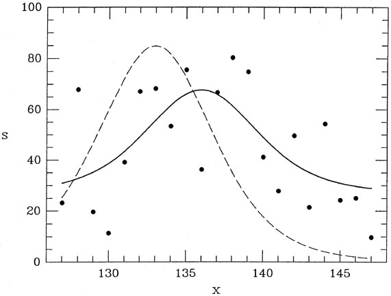
Figure 2-13.