


APERTURE PHOTOMETRY AND SKY DETERMINATION
Before we can perform the final nonlinear least-squares profile fits, we
must first obtain
starting guesses for the remaining unknown parameters: the brightness of
the star and the
local brightness of the sky (we already have decent guesses at the x, y
coordinates of the
centroid, from FIND). In principle, we could derive a starting guess at
the magnitude from
the central  -value of each star,
from FIND. However, we certainly wouldn't want to use
the
-value of each star,
from FIND. However, we certainly wouldn't want to use
the  -value that we could have
gotten from FIND as the sky value, because this estimate is
based on very few pixels, and those few pixels are already known to
contain some significant object.
-value that we could have
gotten from FIND as the sky value, because this estimate is
based on very few pixels, and those few pixels are already known to
contain some significant object.
DAOPHOT's PHOTOMETRY routine gets improved estimates of the brightnesses of star and sky by synthetic aperture photometry. In effect, the software draws a simple, roughly circular, aperture around the estimated position of the star, and the total amount of "light" within the aperture is determined by simply adding up the data numbers. At the same time, the software draws a circular annulus around the position of the star, and builds up the histogram of brightness values found in the pixels in that annulus. PHOTOMETRY presently uses an algorithm originally developed for the "mountain software" package at Kitt Peak to derive a robust estimate of the average sky brightness from this histogram: in an iterative procedure, the mean and standard deviation of the histogram are computed, the tails beyond a certain number of standard deviations from the mean are chopped off, the mean and standard deviation are recomputed, and the process continues until the mean and standard deviation stop changing. The local sky brightness is defined as the estimated mode of this truncated histogram. However, because of Poisson errors the peak of histogram will be ratty, so the literal mode of the distribution, as defined by that brightness value which occurs most frequently, will be rather poorly defined. Furthermore, if your image data are integers, then the literal mode can also only be an integer. In general, this may not be quite as accurate an estimate of the sky value as you want. Therefore the modal value which is actually used is estimated from
(see Fig. 4-3) which - I believe - is strictly
true for a skewed Gaussian. As I said, I
deserve absolutely zero credit for developing this algorithm, but I have
found it works well
and quickly enough that so far I have felt little urge to try to improve
on it. However,
it may be getting to be time to try for an improved sky estimator. I
suspect that some
really clever person could work up a good, robust, precise mode-finder
using something like
the (a, b) weight-fudging scheme which I outlined in the second half of
Lecture 3, and the
expected sky
Why do we want to use the mode of the sky-brightness histogram,
rather than the
mean or the median. Well, think about it. The mode, the peak of the
distribution, is that
location where most of the histogram's volume is contained in the
shortest distance. If you
adopt the mode of the histogram as your estimate of the sky brightness
per pixel, you suffer
the smallest possible probability of making a large error in the sky
brightness of any given
pixel. You don't really want to know what the sky brightness would be if
there were no
stars in the frame, you want to know what the typical sky brightness is
in a pixel with
typical starlight contamination. Then, when this brightness is
subtracted from each pixel
in the small, circular star aperture, the amount of flux remaining is
the most likely estimate
for the net flux due to that star alone, exclusive of the typical
contamination due to the sky and the other stars in the frame.
Obviously the stellar brightness measurement which is obtained here is
still only a
crude approximation of the actual stellar brightness. First of all, the
light of some other
stars may or may not be leaking into the aperture - there will always be
some positive
or negative difference between the "typical" contamination by starlight
in that part of
the frame, and the contamination which actually occurs in that
particular aperture. To
minimize the random errors engendered by this uncertainty, the aperture
cannot be made
very large. Since the aperture is not very large, some of the light of
the star you want to
measure will fall outside the aperture; as a result, you wind up
underestimating the star's
total flux. However, as long as you use the same small aperture for
every star, all stars will
be underestimated by the same fractional amount, and their relative
magnitudes - which
is all you need to get the profile-fitting started - will be OK. How you
recover the flux
which fell outside that small aperture, so that you can place the
magnitudes from this CCD
frame on an absolute photometric system, will be part of my last
lecture.
 which can be
computed from first principles on the basis of the read-noise
and gain of the detector (as distinguished from that
which is
estimated empirically from the observed histogram).
which can be
computed from first principles on the basis of the read-noise
and gain of the detector (as distinguished from that
which is
estimated empirically from the observed histogram).
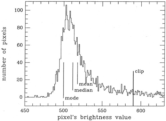
Figure 4-3.