


PROFILE MODELLING
The way in which the point-spread function is encoded is one of the principal details that distinguish the various existing photometric packages from one another. There are two general approaches which have been tried in the past:
(1) Some analytic function of suitable form is fitted to bright,
isolated stars in the
frame - much as we did in the second lecture. The assumed analytic form,
together with
the "best" values of the fitting parameters which result from these
fits, are taken to define
the PSF for the frame, which can then be evaluated at any distance
( x,
y) from the
center of any particular star. Again, referring back to our fits in the
second lecture, the
hypothesis that the stellar profile is exactly described by a circular
Moffat function, plus
the derived values of the parameters
x,
y) from the
center of any particular star. Again, referring back to our fits in the
second lecture, the
hypothesis that the stellar profile is exactly described by a circular
Moffat function, plus
the derived values of the parameters
 and
and
 , tell you
everything you need to know about
a frame's PSF. This PSF can then be fit to all the stars in the frame to
determine their individual values of
, tell you
everything you need to know about
a frame's PSF. This PSF can then be fit to all the stars in the frame to
determine their individual values of
 0,
0,
 0,
0,
 , and
, and
 . More complex analytic equations
involving more
shape parameters can easily be devised to model images that depart from
simple circular
symmetry. This is the approach adopted by ROMAFOT and STARMAN.
. More complex analytic equations
involving more
shape parameters can easily be devised to model images that depart from
simple circular
symmetry. This is the approach adopted by ROMAFOT and STARMAN.
(2) The actual brightness values observed in pixels in and around
the images of bright
stars are assumed to define the frame's PSF empirically; subarrays
containing bright stars
are extracted from the main image, averaged together, and retained as
look-up tables giving relative brightness as a function of
(x,
y) offset from a star's
center. Since the positions
of the stars within the coordinate grid of the original CCD frame will
differ by different
fractional-pixel amounts, if multiple stars are used to define the
frame's PSF they must
be shifted to a common centering within the coordinate grid by numerical
interpolation
techniques before they can be averaged together to form the frame's mean
PSF - otherwise
the model profile will be a bit broader than the true profile. When the
resulting PSF is
fitted to individual program stars, numerical interpolation techniques
must again be used
to shift that PSF to the actual fractional-pixel position of the program
star. This is the approach used by RICHFLD and WOLF.
Each of these approaches has its advantages and disadvantages. The analytic PSF can be comparatively simple to program and use. However, it has the disadvantage that real stellar images are often quite far from circular - or even bilateral - symmetry due to optical aberrations or guiding errors, so it may become necessary to include a fairly large number of shape parameters in the model. ROMAFOT makes complex stellar profiles by adding up however many Moffat functions it needs; STARMAN employs the sum of a tilted Lorentz function and a circular Gaussian, involving some eight (by my count) shape parameters. When this many parameters are involved, they can become rather strongly intertangled: starting guesses for some of the more subtle parameters can be hard to come by, and some manual guidance or a fairly sophisticated set of clamps may be needed to help shepherd the shape determinations to final convergence. Even with all this sophistication, tractable analytic functions still may not provide enough flexibility to model pathological (but real) star images when the data are over-sampled. When a bright star has a full-width at half maximum of, say, 3 pixels, its profile is still often detectable out to a radius of 12 or more pixels: that means the star image may contain some 242 / 32= 64 potentially independent resolution elements. If the telescope tracking and aberrations are bad enough, it could require an analytic function with as many as 64 different shape parameters to fully describe such a profile.
The empirical point-spread function, on the other hand, has by definition essentially one free shape "parameter" for every pixel which is included in the look-up table. However bizarre the stellar profile, provided that it repeats from one star to the next, it will be accurately reproduced in the mean empirical PSF. With so many independent degrees of freedom, empirical PSFs tend to be noisy: if the PSF is derived from a single star, whatever noise existed in that star's own profile will be copied verbatim into the PSF. In contrast, With the analytic PSF the fact that a large number of pixels is used to define a small number of parameters tends to smooth out the noise; with the empirical PSF the noise can be suppressed only by averaging together many stars. A more serious problem for the empirical PSF is that it tends to fall apart when the data become critically sampled or undersampled. In the flanks of a star image in a critically sampled frame the relative intensity may change by nearly an order of magnitude from one pixel to the next. That being the case, it is extremely difficult for any cookbook interpolation scheme (RICHFLD uses splines, WOLF uses sinc interpolation) to achieve ~ 1% accuracy in predicting what the pixel values would have been had the star been centered differently. In contrast, knowledge of the analytic profile being continuous rather than discrete, an analytic profile can be evaluated for any pixel centering.
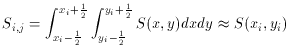
However, when an image is critically sampled or undersampled, it is no longer adequate to estimate the flux contained within a pixel by evaluating some analytic function at the center of that pixel: one must actually integrate the analytic function over the two-dimensional area of the pixel. In mathematical terms, the approximation
is no longer accurate at the ~ 1% level. Now for the empirical
point-spread function, this is
not an extra problem, because the observed brightness values that go
into the look-up table
are already de facto integrals over square subportions of the stellar
profile. However, to fit
an analytic PSF properly to such data, the analytic formula must be
integrated over the
area covered by each individual pixel before it can be properly compared
to the brightness
observed in that pixel. Since for complex formulae no simple analytic
integral may exist,
these integrations must in general be performed numerically. This can
greatly increase the execution time.
In writing DAOPHOT, I decided to try to use that blend of analytic and
empirical
profiles which would best suit the kind of data that my colleagues and I
were trying to
reduce. Let me place things in context: some of our data were obtained
with the Cerro
Tololo and Kitt Peak telescopes. The CCDs we used there had scales of
The obvious thing to do, then, was to use an empirical look-up table:
this is the best
way to map out any complexities in an oversampled profile that are
produced by tracking
errors and aberrations. However, on those occasions when our data did
approach critical sampling, it was found that the inadequate
interpolations added unacceptable noise to the
fits. Therefore I adopted a hybrid point-spread function for
DAOPHOT. First, the pixel-by-pixel
integral of a simple analytic formula is fit by non-linear least squares
to the data for
the bright, isolated PSF stars. Then, all the stars' residuals from this
fit are interpolated
to a common grid, and averaged together into a look-up table. When this
hybrid PSF is
evaluated to fit some pixel in the image of a program star, first the
best-fitting analytic
formula is integrated over the area of that pixel, and then a correction
from that analytic
profile to the true model profile is obtained by interpolation in the
look-up table of residuals.
What does this buy us? Well, as I said earlier, when the data are
critically-to-over-sampled,
it is difficult for a simple analytic formula to represent a real star
image with an
accuracy of order 1%. However, a well-chosen formula can represent a
stellar profile with
a pixel-to-pixel root-mean-square residual of order 5% (give or take,
plus or minus, pro or
con). By first fitting and subtracting this best analytic model, the
values that I put into
the look-up table are of order 20 times smaller than would have been the
case had I put the
raw observed intensities themselves into the table. As a result, the
absolute errors caused
by the inadequate interpolation are also of order 20 times smaller than
they would have been.
There's another way of looking at this. When you use some numerical
interpolation
scheme, you are making implicit assumptions about the variations in the
stellar profile
between the sample points. If you use cubic-spline interpolation, you
are saying that
the fourth and all higher derivatives of the profile are identically
zero. If you use sinc
interpolation, you are saying that in the profile all spatial
frequencies higher than the
Nyquist frequency are identically zero. Neither of these assumptions is
adequate for
critically sampled star images. By combining an analytic first
approximation with cubic-spline
interpolation within a look-up table of corrections, I am saying that
the first three
derivatives of the stellar profile can be anything, but the fourth and
all higher derivatives
are precisely those of the analytic approximation. Had I used sinc
interpolation within the
table of corrections, I would have been saying that all spatial
frequencies below the Nyquist
frequency could be anything, but all frequencies above the Nyquist
frequency would be those of the analytic approximation.
As I just implied, I adopted cubic-spline interpolation rather than sinc
interpolation
to evaluate the empirical correction from the analytic approximation to
the true model
profile. For the analytic approximation, I adopted the Gaussian
function. A Gaussian
function is not a particularly good match to a real stellar profile, and
if you were to write
a program to fit purely analytic model profiles to real star images, I
would advise strongly
against using Gaussians; a Moffat function, as used by ROMAFOT, or some
superposition
of Gaussian plus power law, as used by STARMAN, would be much
better. However, as I
will discuss in more detail tomorrow, the Gaussian function is believed
to be a pretty good
description of the central part of the stellar profile, where
things are changing rapidly with
position, while the non-Gaussian wings - which have small high-order
derivatives (=> small
amplitudes at high spatial frequencies) can be adequately mapped in the
look-up table of
corrections. Moreover, the Gaussian function does have one other -
highly desirable - advantage:
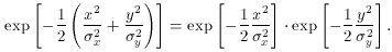
a two-dimensional Gaussian function can be separated into the product of two
one-dimensional Gaussians:
Now, rather than having to compute a two-dimensional numerical integral
over the area of
each pixel, I can compute two one-dimensional integrals and multiply
them together. This
turns out to cut the reduction time in half. Maybe a mere factor of two
doesn't seem like
very much, but if you could get exactly the same answer with half the
work, wouldn't you
do it? And you do get effectively the same answer, as long as the data
are at least critically sampled.
However, as the years have passed, we have started getting undersampled images.
We've had some really good seeing at Cerro Tololo, and at the prime
focus of the Canada-France-Hawaii
telescope it's not rare to get 0".6 seeing, with 0".4 pixels. It turns out that
when you are significantly undersampled (FWHM
 O".6 per pixel,
and the seeing was seldom as good as 1"; 1".2 to 1".8 was more
typical. Thus, these data
ranged from critically sampled to slightly oversampled. The rest of our
data were obtained
at the cassegrain focus of the Canada-France-Hawaii telescope, with a
scale of O".2 per pixel,
and seeing typically O".6 - 1".2; these data were thus somewhat oversampled.
O".6 per pixel,
and the seeing was seldom as good as 1"; 1".2 to 1".8 was more
typical. Thus, these data
ranged from critically sampled to slightly oversampled. The rest of our
data were obtained
at the cassegrain focus of the Canada-France-Hawaii telescope, with a
scale of O".2 per pixel,
and seeing typically O".6 - 1".2; these data were thus somewhat oversampled.
 1.5 pixels, say), the
look-up table of
corrections can no longer absorb all of the difference between a
Gaussian function and a
real stellar profile: the Gaussian is just too wrong. The easiest
solution is simply to use
an analytic function which looks more like a real star, so that the
residuals the look-up
table must handle are smaller. Accordingly, I am just starting work on a
new generation
of DAOPHOT which will offer the user a choice of analytic first
approximations, including
the old, standard Gaussian; a Moffat function, like ROMAFOT's; and a
"Penny" function
(a superposition of a Gaussian and a Lorentzian), like STARMAN's. The
Gaussian can be
used for critically sampled and oversampled data, where you get the
factor of two increase
in speed with no appreciable loss of precision. The Moffat function or
the Penny function
can be used for undersampled data; these reductions will take longer,
but there should be
minimal loss of precision due to inadequate interpolations.
1.5 pixels, say), the
look-up table of
corrections can no longer absorb all of the difference between a
Gaussian function and a
real stellar profile: the Gaussian is just too wrong. The easiest
solution is simply to use
an analytic function which looks more like a real star, so that the
residuals the look-up
table must handle are smaller. Accordingly, I am just starting work on a
new generation
of DAOPHOT which will offer the user a choice of analytic first
approximations, including
the old, standard Gaussian; a Moffat function, like ROMAFOT's; and a
"Penny" function
(a superposition of a Gaussian and a Lorentzian), like STARMAN's. The
Gaussian can be
used for critically sampled and oversampled data, where you get the
factor of two increase
in speed with no appreciable loss of precision. The Moffat function or
the Penny function
can be used for undersampled data; these reductions will take longer,
but there should be
minimal loss of precision due to inadequate interpolations.