


3.4 The Minimum Chi-Square Method
The method is an extension of the chi-square goodness-of-fit test described in Section 4.2. It will be seen that it is closely related to least squares and weighted least squares methods; the minimum chi-square statistic has asymptotic properties similar to ML. Pearson's (1900) paper in which it was introduced is a foundation stone of modern statistical analysis (4); a comprehensive and readable review (plus bibliography) was given by Cochran (1952).
Consider observational data which can be binned, and a model/hypothesis which predicts the population of each bin. The chi-square statistic describes the goodness-of-fit of the data to the model. If the observed numbers in each of k bins are Oi, and the expected values from the model are Ei, then this statistic is
(The parallel with weighted least squares is evident: the statistic is
the summed squares of the residuals weighted by what is effectively
the variance if the procedure is governed by Poisson statistics.) The
null hypotheses H0 (see
Section 4.1) is that
the proportion of objects falling in each category is
Ei; the chi-square procedure tests whether
the Oi are sufficiently close to Ei
to be likely to have occurred
under H0. The sampling distribution under
H0 of the statistic
Fig. 4. The
The premise of the chi-square test then is that the deviations from
Ei are due to statistical fluctuations from limited
numbers of
observations per bin, i.e. ``noise'' or Poisson statistics, and the
chi-square distribution simply gives the probability that the chance
deviations from Ei are as large as the observations
Oi imply.
There is good news and bad news about the chi-square test. First the
good: it is a test of which most scientists have heard, with which
many are comfortable, and from which some are even prepared to accept
the results. Moreover, because
Now the bad news: the data must be binned to apply the test, and the
bin populations must reach a certain size because it is obvious that
instability results as Ei -> 0. As another rule of
thumb then: > 80 per
cent of the bins must have Ei > 5. Bins may have to be
combined to
ensure this, an operation that is perfectly permissible for the
test. However, the binning of data in general, and certainly the
combining of bins, results in loss of efficiency and information,
resolution in particular.
The minimum chi-square method of model-fitting consists of
minimizing the
The essential question, having found appropriate parameters, is to
estimate confidence limits for them. The answer is as given by
Avni (1976):
the region of confidence (significance level
where
[It is interesting to note that (a) the
By way of example, see Fig. 5. The model to
describe the distribution (Fig. 5a) requires
two parameters,
Fig. 5. An example of model-fitting via the
minimum-
A last comment on the method of minimum chi-square. The procedure
has its limitations - loss of information due to binning and
inapplicability to small samples. However, it has one great advantage
over other model-fitting methods - the test of the optimum model is
carried out for free, as part of the procedure. For instance, the
example of Fig. 5 - there are seven bins, two
parameters and the
appropriate number of degrees of freedom is therefore four. The value
of
 2
follows the chi-square distribution (Fig. 4)
with v = (k - 1) degrees
of freedom. Table A III presents critical
values; if 2 exceeds these
values, H0 is rejected at that level of significance.
2
follows the chi-square distribution (Fig. 4)
with v = (k - 1) degrees
of freedom. Table A III presents critical
values; if 2 exceeds these
values, H0 is rejected at that level of significance.
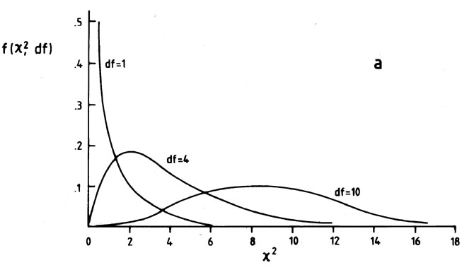
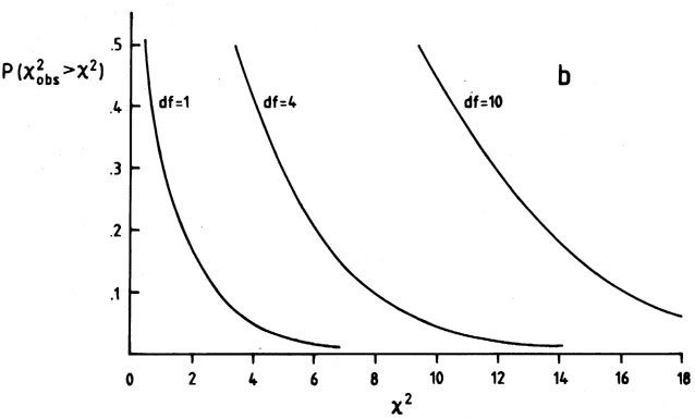
2 distribution. (a) f (2, df), the probability density
function of 2 for
df degrees of freedom. (b) The distribution
function  2
2 2, df) d2 of Table III,
consulted to
determine if 2 is
``too large'' for a good fit, or ``large enough'' to reject
H0.
2, df) d2 of Table III,
consulted to
determine if 2 is
``too large'' for a good fit, or ``large enough'' to reject
H0.
 ) above minimum
Number of parameters
Significance

1 2 3
0.68 1.00 2.30 3.50
0.90 2.71 4.61 6.25
0.99 6.63 9.21 11.30
2 is additive, the results of
different data sets which may fall in different bins, bin sizes, or
which may apply to different aspects of the same model, may be tested
all at once. The contribution to 2 of each bin may be examined and
regions of exceptionally good or bad fit delineated. In addition, 2
is easily computed, and its significance readily estimated as
follows. The mean of the chi-square distribution equals the number of
degrees of freedom, while the variance equals twice the number of
degrees of freedom; see plots of the function in
Fig. 4. So as another
rule of thumb, if 2 should come out (for more than four bins) as
~ (number of bins - 1) then accept H0. But if 2 exceeds twice (number
of bins - 1), H0 will probably be rejected.
2 statistic by varying the parameters of the
model. The premise on which this technique is based is obvious from
the foregoing - the model is assumed to be qualitatively correct, and
is adjusted to minimize (via 2) the differences between the Ei
and Oi
which are deemed to be due solely to statistical fluctuations. In
practice, the parameter search is easy enough (with computers) as long
as the number of parameters is less than four; if four or more, then
sophisticated search procedures may be necessary. The appropriate
number of degrees of freedom to associate with 2 is [k - 1 - (number of parameters)].
) is defined by
 is from
Table 1.
depends only on the number
of parameters involved, and not on the goodness-of-fit (2min) actually
achieved, and (b) there is an alternative answer given by
Cline & Lesser (1970)
which must be in error: the result obtained by Avni has
been tested with Monte Carlo experiments by Avni himself and by
M. Birkinshaw (personal communication).]
is from
Table 1.
depends only on the number
of parameters involved, and not on the goodness-of-fit (2min) actually
achieved, and (b) there is an alternative answer given by
Cline & Lesser (1970)
which must be in error: the result obtained by Avni has
been tested with Monte Carlo experiments by Avni himself and by
M. Birkinshaw (personal communication).]
 and k. Contours of
2 resulting from the
parameter search are shown in Fig. 5(b). When
the Avni prescription is applied, it gives 20.68 = 2min + 2.30, for
the value corresponding to 1
and k. Contours of
2 resulting from the
parameter search are shown in Fig. 5(b). When
the Avni prescription is applied, it gives 20.68 = 2min + 2.30, for
the value corresponding to 1 (significance level = 0.68); the contour
20.68 = 6.2
defines a region of confidence in the (, k) plane
corresponding to the 1 level of
significance. (Because the range of
interest for was
limited from other considerations to 1.9 < < 2.4,
the parameter search was not extended to define this contour fully.) A
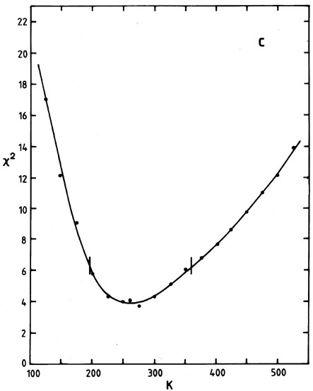
cut along a line of constant is shown in Fig. 5(c); the calculation
of 2 defines upper and
lower values of k corresponding to = 1 for
this particular .
(significance level = 0.68); the contour
20.68 = 6.2
defines a region of confidence in the (, k) plane
corresponding to the 1 level of
significance. (Because the range of
interest for was
limited from other considerations to 1.9 < < 2.4,
the parameter search was not extended to define this contour fully.) A
cut along a line of constant is shown in Fig. 5(c); the calculation
of 2 defines upper and
lower values of k corresponding to = 1 for
this particular .
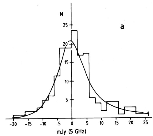
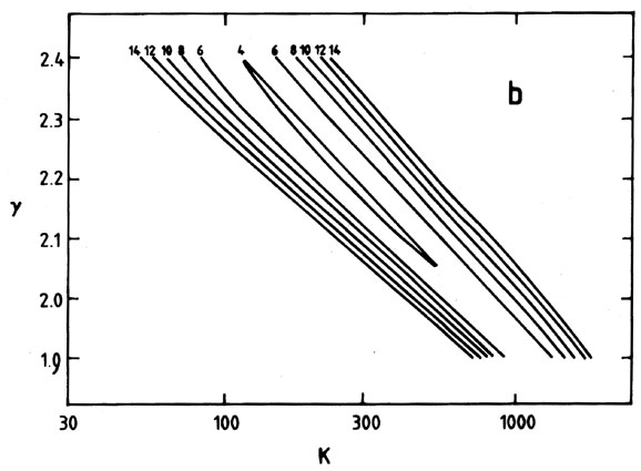
2 technique. The
object of the experiment was to obtain a series of radio
background-deflection measurements from which to determine parameters
describing the number count [N (S) relation] of faint extragalactic
sources at 5 GHz. A power-law form N = kS was assumed, the
parameters and
K to be determined. (a) Binned observations of the
background deflections measured. The smooth curve shows the optimum
model found from the minimum-2 procedure. (b) Contours of 2 in the
(, K) plane
for the data of (a). (c) A cut through the (, K) plane
at constant = 2.2
showing the ± 68.3 per cent or 1 confidence limits.
2min is
about 4, just as one would have hoped, and the optimum
model is thus a satisfactory fit.
4 Pearson's paper is entitled On the
criterion that a given system of
deviations from probable in the case of a correlated system of
variables is such that it can be reasonably supposed to have arisen
from random sampling. It is wonderful polemic and gives several
examples of the previous abuse of statistics, covering the frequency
of buttercup petals to the incompetence of Astronomers
Royal. (``Perhaps the greatest defaulter in this respect is the late
Sir George Biddell Airy . . . .'') He demonstrates, for extra measure, that
a run of bad luck at his roulette wheel, Monte Carlo, in 1892 July had
1 chance in 1029 of arising by chance; he avoids any libel by
phrasing
his conclusion ``. . . . it will be more than ever evident how little
chance had to do with the results . . .''. Back.