B. The Cosmic Background Anisotropies

The discovery of the anisotropies in the cosmic background by COBE created a new opportunity for verification of cosmological parameters and theories of large-scale formation. As discussed at the beginning of this paper, the CMB offers a `snap-shot' of the universe at the time of recombination (z ~ 1000). The anisotropies that were present in the baryon-photon plasma at this time are manifested today by the temperature fluctuations in the spectrum. These fluctuations are representative of a nearly Gaussian, scale-invariant spectrum. As discussed previously, this is a unique prediction of inflation theories.

Although the quantitative details can become formible, the qualitative description of these temperature fluctuations is quite simple. During inflation, the perturbations formed must be of nearly the same amplitude and randomly distributed, as discussed above. After reheating takes place, these classical perturbations re-enter the horizon causing density fluctuations in the baryon-photon plasma. In over-dense regions, potential wells form that trap the plasma and cause it to heat up. At the same time, photon pressure induces a kind of restoring force to oppose the gravitational potential. In this way, a harmonic oscillator motion is set up in the plasma. These oscillations continue with no friction (viscosity) from the fluid. This is why they are referred to as adiabatic fluctuations. However, if this were not the case and the friction is deemed important, one obtains an isocurvature spectrum [64]. These turn out to be indicative of cosmic strings, which are ruled-out by observation as a method of primordial structure formation. However, models containing cosmic strings that are produced during reheating following inflation may still play a major role in cosmological models [65].

At the time of recombination, when the photons were able to escape the fluid, they had to overcome the gravitational potentials. The picture is that the photons in these potential wells were hotter than the average, but this temperature difference was partially cancelled by the gravitational redshift resulting from the photons `climbing' out of the potential well. This phenomena is know as the Sachs-Wolf effect. The result is that the photons that were in the wells have a slight temperature increase from those that were not. This variation is predicted by theory to be on the order of 10^-5 [22]. These oscillations propagate through the fluid at the speed of sound. Thus, there is a acoustic horizon that is generated within the surface of last scattering and if present today would have an angular size of about one degree on the sky.

One concern with the simplicity of this analysis is what effects, such as reionization in the surface of last scattering, must be considered? It is important to consider the mean free path of the photon as it travels within the fluid before escaping. This could affect the energy and therefore temperature of the spectrum. However, it turns out that this effect only appears on small angular scales within the spectrum and can be ignored [58]. Also, any effects from CMB scattering off interstellar gas only appear in the spectrum at very small angles. These observations are of course useful, but offer little insight into examination of the early universe and formation of large-scale structure.

Given the predicted anisotropies from the Sachs-Wolf effect, the next step is to examine the cosmic background spectrum through observation. The anisotropies in the temperature of the cosmic background spectrum can be expanded in spherical harmonics [56],

(84)

The multipole coefficients are given by,

(85)

The amount of anisotropy at multipole moment l is expressed by the power spectrum,

(86)

The C_l's measure the temperature anisotropy of two regions separated by angle . This angle is related to the l's by: ~ 180° / l. Thus, l allows one to express the temperature variations of regions separated by an angle 180° / l. The l = 0 represents the monopole contribution to the anisotropy, which is of course zero (this is comparing a point separated from itself by 360°. The next moment, l = 1, is the dipole moment, which compares regions separated by 180°. This anisotropy originates from our peculiar velocity, the motion of the Earth relative to the cosmic background. This moment is usually taken out of the spectrum to leave the `true' anisotropy. The l = 2 moment is the quadrupole contribution, which marks the first non-trivial anisotropy for understanding structure formation.

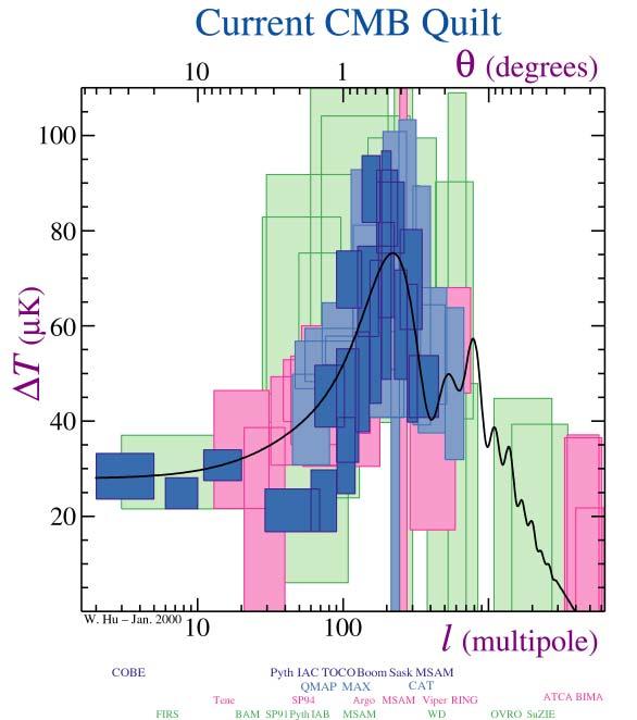
When the COBE data is plotted with multipole l versus temperature variation, a peak is found to occur around l = 220 or 1° (Figure (10)). This peak corresponds to the angular size on the sky of the acoustic horizon discussed before and has been called the Doppler peak. Thus, there is a maximum temperature variation at precisely the angle predicted by the Sachs-Wolf effect. Since a mechanism of this type can only be explained by an inflationary model, one is presented with a strong argument for inflation [64].

Figure 10. Power Spectrum Plot of the Cosmic Background - The data is normalized to the quadrupole (l = 2) anisotropy detected by COBE. The Doppler peak corresponds to a maximum power fluctuation at a multipole of l = 220, which is about an angle of one degree on the sky. This graph provided by Wayne Hu [64].

To examine one aspect of the complexity involved, consider that the scalar and tensor perturbations can be fixed by their contribution to the quadrupole moment C_l=2 of the CMB [66].

(87)

(88)

where V = V() is the inflaton potential, S is the scalar contribution, and T is the tensor contribution. When the slow-roll approximation is considered and the determination of cosmological parameters is found by methods other than CMB analysis; e.g., for large-scale structure probing, one finds that the ratio T/S is less than order unity. This restricts V 5 x 10^-12. Reformulating equation (82) in terms of the inflaton potential, one finds in Planckian units the relations for the scalar and tensor spectral indices, respectively.

(89)

(90)

Although most models of inflation predict a near scale-invariant, or Harrison-Zel'dovich spectrum, the small deviations from differing potentials V() give a way of testing inflation models. With future experiments such as MAP ⁽²⁸⁾ and PLANCK ⁽²⁹⁾ , these spectral indices will be found with great precision and the shape and height of the spectrum can be used to manifest the correct inflaton potential. In this way, inflation will be used to predict new particle physics, instead of the original scenario which was vice versa.

However, the ultimate test of inflation is the precise determination of the tensor perturbations, that is the n_t's. This can't be deduced from the CMB spectrum because both the scalar and tensor perturbations contribute to the temperature anisotropy. However, if a method could be devised to separate out the tensor perturbations and this spectrum were detected, it would be concrete evidence of an inflationary period. This is because inflation is the only way metric perturbations can survive to the present. This is due to the structure of a DeSitter spacetime.

The tensor spectrum can be separated by creating a polarization map of the CMB. The separation is then possible because the tensor perturbations have an intrinsic axial component, and the angular dependence can be determined from the metric. Whereas, the scalar perturbations have no dependence on direction. Therefore, the polarization vector can be constructed out of two parts, a curl and a gradient.

(91)

where gives the direction. Thus, to obtain the tensor terms one can take the divergence of this vector. Before proceeding further, it may be of interest to the reader why the perturbations only contain tensor and scalar contributions and vector type perturbations are absent. This is because massless vector fields are conformally invariant [67]. This invariance can be broken by introducing a mass term or by explicitly breaking the coupling. Although for a massive vector field the perturbations generated are far too small and die off far too quickly during the inflationary expansion [68]. Thus, a standard prediction of inflation is that there are no vector perturbations. But, isn't the polarization a vector? No. The polarization is actually a 2 x 2 trace free symmetric tensor. This tensor is written in terms of the Stokes parameters Q() and U(), which give us the polarization in each direction. For an explanation of these parameters see, [69, section 7.2].

(92)

The polarization tensor can be expanded in tensor spherical harmonics [70],

(93)

The Y^G_(lm)ab and Y^C_(lm)ab represent a basis for the gradient (scalar) and curl (tensor) perturbation terms in this polarization mapping. The a^G_(lm)'s and a^C_(lm)'s are again just found by exploiting the orthogonality. One can use this spectrum to construct necessary requirements for the potentials of the inflaton field and this analysis can therefore be used to distinguish the various inflation models.

²⁸ http://map.gsfc.nasa.gov. Back.
²⁹ http://astro.estec.esa.nl/SA-general/Projects/Planck. Back.