


C. Summary
Scalar perturbations are the most easily detected form of perturbation. The scalar nature of these fluctuations arise from the fact that the perturbations are of mass fields in the primordial era, that is, before the time of decoupling. Different models of inflation and the corresponding reheating mechanisms differ in their predictions of mass variation. Regardless, these variations of the early universe eventually give rise to the structural formation of galaxy clusters, which can help distinguish the various theories of inflation and structure formation. Tensor perturbations are also detectable and these perturbations result from fluctuations in the space-time metric in the primordial era. Again, these perturbations are very small and would be very hard to detect. However, certain models of inflation predict wavelengths that could be detected by laser interferometry gravitational wave detectors, such as LIGO (30) If these waves were detected it would help eliminate many inflation models and help narrow the region of viable theories. Furthermore, inflation is the only theory that can currently account for a gravitational wave spectrum. The detection of the spectrum would be a great success for the inflation theory.
Both of these types of perturbations contribute to the 10-5 temperature fluctuation in the cosmic background. The biggest challenge for experimentalists is to separate the scalar and tensor contributions to the temperature fluctuations. In practice this is very difficult, if not impossible, and it becomes more practical to consider the polarization of the CBR.
For the inflationist, the goal of CRB measurements is to
distinguish between the various models of inflation. A good way
to begin, is to express many of the relations obtained thus far,
in terms of  and
and
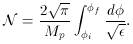
 . The number of e-foldings
(N) can be expressed in terms of
using
(63) and (78),
. The number of e-foldings
(N) can be expressed in terms of
using
(63) and (78),
Another useful relation, which may be found in the literature
[61],
gives a measure of when a given perturbations of
wave length k passes through the horizon and is therefore
`frozen out'. This can be expressed as the number of e-foldings
N(k) from the end of inflation.
Vk is the potential when the mode k leaves the
horizon,
Ve is the potential at the end of inflation, and
With the rapid advances in observational cosmology, cosmologists
are able to use the abundance of data that is being obtained by
the Hubble Space Telescope, balloon experiments, satellites (such
as Chandra), etc. to narrow the parameters of the universe. Then
with these values and the relations that have been presented in
this section, one can use inflation to predict new physics for the
pre-inflation or Planckian epoch. Ultimately this physics will
need a quantum theory of gravity or supersting theory, but
determination of the inflaton potential and the resulting
large-scale structure will set stringent limits in which to test
the predictions of these new theories. In this way, inflation
offers the link between the innerspace of the quantum realm and
the outerspace of the large-scale structure of the universe. The
marvelous universe in which we live, the beauty that surrounds us,
and even ourselves, will be the result of a quantum fluctuation or
perhaps a chaotic mishap.
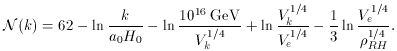
 RH
is the energy density after reheating. This expression may appear
formidable, however it can be used to begin understanding density
fluctuations. For example, the modes k entering the horizon
today, left the horizon at N(k) = 50-70. The
uncertainty in this range manifests the lack of knowledge of the
inflaton potential. Thus, once again different inflaton models
make different predictions.
RH
is the energy density after reheating. This expression may appear
formidable, however it can be used to begin understanding density
fluctuations. For example, the modes k entering the horizon
today, left the horizon at N(k) = 50-70. The
uncertainty in this range manifests the lack of knowledge of the
inflaton potential. Thus, once again different inflaton models
make different predictions.