Copyright © 1992 by Annual Reviews. All rights reserved
| Annu. Rev. Astron. Astrophys. 1992. 30:
499-542 Copyright © 1992 by Annual Reviews. All rights reserved |


3.3 Distance Measures
As we look out from our self-defined position at r = 0 to observe some object at a radial coordinate value r1, we are also looking back in time to some time t1 < t0, and back to some expansion factor R1 = R(t1) that is smaller than the current value R0. Note, however, that neither r1, t1, nor R1 are directly measurable quantities. Rather, the measurable quantities are things like the redshift z; the angular diameter distance
where D is a known (or assumed) proper size of an object and
where u is a known (or assumed) transverse proper velocity and
where
One sees in particular that dA, dM,
and dL are not independent, but related by
independent of the dynamics of R(t). This is perhaps a disappointment,
since it means that we cannot learn anything about
Looking back along a light ray, R, r, and t are
related by the
equation for a radial, null geodesic of the Friedmann-Robertson-Walker
metric, namely
Multiplying this equation by R0, and using Equations
22 and 16, and
the definitions of
where ``sinn'' is now defined as sinh if
Figure 5. Angular diameter distance as a
function of redshift for
models A-E. Objects of a small fixed z look farther away (have smaller
angular diameters) in

 is its
apparent angular size; the proper motion distance
is its
apparent angular size; the proper motion distance

 is an
apparent angular motion; and the luminosity distance
is an
apparent angular motion; and the luminosity distance
 is a known (or
assumed) rest-frame luminosity and
is a known (or
assumed) rest-frame luminosity and
 is an
apparent flux. The relation of the measurables to the unmeasurables
turns out to be
(Lightman et al 1975,
Section 19.9)
is an
apparent flux. The relation of the measurables to the unmeasurables
turns out to be
(Lightman et al 1975,
Section 19.9)

 M,
M,
 simply by
comparing two distance indicators of a single object. Rather, the
information about M,
is contained in the
dependence of the
distance indicators on redshift z, which we now calculate.
simply by
comparing two distance indicators of a single object. Rather, the
information about M,
is contained in the
dependence of the
distance indicators on redshift z, which we now calculate.
 k
and z, one obtains the integral formula for the
distance measure at redshift z,sub>1,
k
and z, one obtains the integral formula for the
distance measure at redshift z,sub>1,
 k > 0 (open
universe) and as
sin if k <
0. Remember that k
is not independent, but given by
Equation 3. (Tn the flat case of
k = 0, i.e.
tot = 1, the sinn and
ks disappear from
Equation 25, leaving only the integral.) The
integral in Equation 25 can be done analytically in the usual special
cases = 0 and
tot = 1 (see
Weinberg 1972 and
Kolb & Turner 1990),
but in general is straightforward to evaluate numerically. Because of
the dependence on k
= 1 - tot in the
sinn function, the qualitative
behavior of Equation 25 is not completely obvious by inspection. At
fixed tot, or when
= 0, the distance measures
all increase with
decreasing M, for
all z. For fixed
M, however, there is no
monotonicity as is increased: The distance
measure will generally
increase at small redshifts, but decrease at redshifts greater than
some particular value. Figure 5 illustrates
these effects for the
specific models A-E. For clarity we plot
d instead
of dM because the
extra factor of (1 + z)-1 (Equation 23) spreads the curves
apart.
k > 0 (open
universe) and as
sin if k <
0. Remember that k
is not independent, but given by
Equation 3. (Tn the flat case of
k = 0, i.e.
tot = 1, the sinn and
ks disappear from
Equation 25, leaving only the integral.) The
integral in Equation 25 can be done analytically in the usual special
cases = 0 and
tot = 1 (see
Weinberg 1972 and
Kolb & Turner 1990),
but in general is straightforward to evaluate numerically. Because of
the dependence on k
= 1 - tot in the
sinn function, the qualitative
behavior of Equation 25 is not completely obvious by inspection. At
fixed tot, or when
= 0, the distance measures
all increase with
decreasing M, for
all z. For fixed
M, however, there is no
monotonicity as is increased: The distance
measure will generally
increase at small redshifts, but decrease at redshifts greater than
some particular value. Figure 5 illustrates
these effects for the
specific models A-E. For clarity we plot
d instead
of dM because the
extra factor of (1 + z)-1 (Equation 23) spreads the curves
apart.
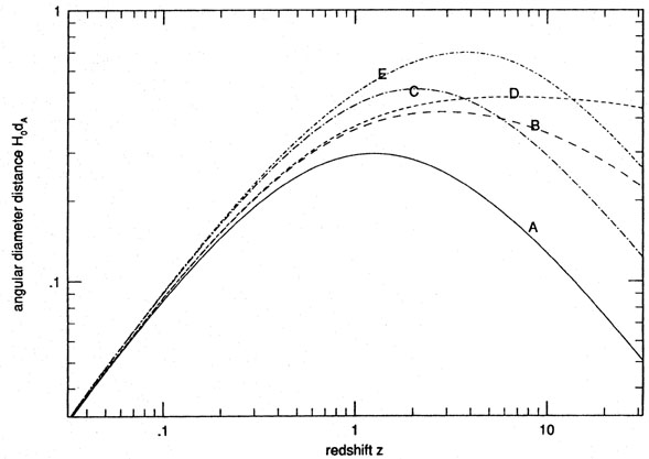
-dominated models. At larger redshifts the
situation reverses. Correspondingly, a fixed angular beam subtends, at
high redshift, a smaller scale for -dominated models than for open
models, giving smaller cosmic microwave background fluctuations for
the -dominated case.