astro-ph/0103017

Abstract. I review the standard paradigm for understanding the formation and evolution of cosmic structure, based on the gravitational instability of dark matter, but many variations on this basic theme are viable. Despite the great progress that has undoubtedly been made, steps are difficult because of uncertainties in the cosmological parameters, in the modelling of relevant physical processes involved in galaxy formation, and perhaps most fundamentally in the relationship between galaxies and the underlying distribution of matter. For the foreseeable future, therefore, this field will be led by observational developments allowing model parameters to be tuned and, hopefully, particular scenarios falsified. In these lectures I focus on two ingredients in this class of models: (i) the role of galaxy bias in interpreting clustering data; and (ii) the statistical properties of the initial fluctuations. In the later case, I discuss some ideas as to how the standard assumption - that the primordial density fluctuations constitute a Gaussian random field - can be tested using measurements galaxy clustering and the cosmic microwave background.

Keywords: cosmology, large-scale structure of the Universe, galaxy formation

Table of Contents

INTRODUCTION

COSMOLOGICAL STRUCTURE FORMATION

Basics of the Big Bang

Linear Perturbation Theory

Primordial density fluctuations

The transfer function

Beyond linear theory

Models of structure formation

OBSERVATIONAL PROSPECTS

Redshift surveys

The Galaxy Power-spectrum

The abundances of objects

High-redshift clustering

Higher-order Statistics

Peculiar Motions

Gravitational Lensing

The Cosmic Microwave Background

TESTING COSMOLOGICAL GAUSSIANITY

Fourier Description of Cosmological Density Fields

The Bispectrum and Phase Coupling

Visualizing and Quantifying Phase Information

BIAS AND HIERARCHICAL CLUSTERING

Hierarchical Clustering

Local Bias

Halo Bias

Progress on Biasing

DISCUSSION

REFERENCES

1. INTRODUCTION

The local Universe displays a rich hierarchical pattern of galaxy clusters and superclusters [Shectman et al. 1996]. The early Universe, however, was almost smooth, with only slight ripples seen in the cosmic microwave background radiation [Smoot et al. 1992]. Models of the evolution of structure link these observations through the effect of gravity, because the small initially overdense fluctuations attract additional mass as the Universe expands [Peebles 1980]. During the early stages, the ripples evolve independently, like linear waves on the surface of deep water. As the structures grow in mass, they interact with other in non-linear ways, more like nonlinear waves breaking in shallow water.

The expansion of the Universe renders the cosmological version of gravitational instability very slow, a power-law in time rather the exponential growth that develops in a static background. This slow rate has the important consequence that the evolved distribution of mass still retains significant memory of the initial state. This, in turn, has two consequences for theories of structure formation. One is that a detailed model must entail a complete prescription for the form of the initial conditions, and the other is that observations made at the present epoch allow us to probe the primordial fluctuations and thus test the theory.

Cosmology is now poised on the threshold of a data explosion which, if harnessed correctly, should yield a definitive answer to the question of initial fluctuations. The next generation of galaxy survey projects will furnish data sets capable answering many of the outstanding issues in this field including that of the form of the initial fluctuations. Planned CMB missions, including the Planck Surveyor, will yield higher-resolution maps of the temperature anisotropy pattern that will subject cosmological models to still more detailed scrutiny.

In these lectures I discuss the formation of large-scale structure from a general point of view, but emphasizing two of the most important gaps in our current knowledge and suggesting how these might be answered if the new data can be exploited efficiently. I begin with a general review of the theory in Section 2, discuss (briefly) possible observational developments in Section 3. Section 4 addresses the form and statistics of primordial density perturbations, particularly the question whether they are gaussian. In Section 5 I discuss uncertainties in the relationship between the distribution of galaxies and that of mass and some recent developments in the understanding of that relationship in a statistical sense.

2. COSMOLOGICAL STRUCTURE FORMATION

The Big Bang theory is built upon the Cosmological Principle, a symmetry principle that requires the Universe on large scales to be both homogeneous and isotropic. Space-times consistent with this requirement can be described by the Robertson-Walker metric

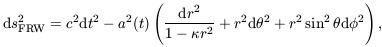
(1)

where is the spatial curvature, scaled so as to take the values 0 or ± 1. The case = 0 represents flat space sections, and the other two cases are space sections of constant positive or negative curvature, respectively. The time coordinate t is called cosmological proper time and it is singled out as a preferred time coordinate by the property of spatial homogeneity. The quantity a(t), the cosmic scale factor, describes the overall expansion of the universe as a function of time. If light emitted at time t_e is received by an observer at t₀ then the redshift z of the source is given by

(2)

The dynamics of an FRW universe are determined by the Einstein gravitational field equations which become

	(3)
	(4)
	(5)

These equations determine the time evolution of the cosmic scale factor a(t) (the dots denote derivatives with respect to cosmological proper time t) and therefore describe the global expansion or contraction of the universe. The behaviour of these models can further be parametrised in terms of the Hubble parameter H = / a and the density parameter = 8 G / 3H², a suffix 0 representing the value of these quantities at the present epoch when t = t₀.

2.2. Linear Perturbation Theory

In order to understand how structures form we need to consider the difficult problem of dealing with the evolution of inhomogeneities in the expanding Universe. We are helped in this task by the fact that we expect such inhomogeneities to be of very small amplitude early on so we can adopt a kind of perturbative approach, at least for the early stages of the problem. If the length scale of the perturbations is smaller than the effective cosmological horizon d_H = c / H₀, a Newtonian treatment of the subject is expected to be valid. If the mean free path of a particle is small, matter can be treated as an ideal fluid and the Newtonian equations governing the motion of gravitating particles in an expanding universe can be written in terms of x = r / a(t) (the comoving spatial coordinate, which is fixed for observers moving with the Hubble expansion), v = - Hr = a (the peculiar velocity field, representing departures of the matter motion from pure Hubble expansion), (x, t) (the peculiar Newtonian gravitational potential, i.e. the fluctuations in potential with respect to the homogeneous background) and (x, t) (the matter density). Using these variables we obtain, first, the Euler equation:

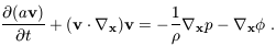
(6)

The second term on the right-hand side of equation (6) is the peculiar gravitational force, which can be written in terms of g = - _x / a, the peculiar gravitational acceleration of the fluid element. If the velocity flow is irrotational, v can be rewritten in terms of a velocity potential _v: v = - _{x v} / a. Next we have the continuity equation:

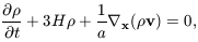
(7)

which expresses the conservation of matter, and finally the Poisson equation:

(8)

describing Newtonian gravity. Here ₀ is the mean background density, and

(9)

is the density contrast.

The next step is to linearise the Euler, continuity and Poisson equations by perturbing physical quantities defined as functions of Eulerian coordinates, i.e. relative to an unperturbed coordinate system. Expanding , v and perturbatively and keeping only the first-order terms in equations (6) and (7) gives the linearised continuity equation:

(10)

which can be inverted, with a suitable choice of boundary conditions, to yield

(11)

The function f ₀^0.6; this is simply a fitting formula to the full solution [Peebles 1980]. The linearised Euler and Poisson equations are

	(12)
	(13)

|v|, ||, || << 1 in equations (11), (12) & (13). From these equations, and if one ignores pressure forces, it is easy to obtain an equation for the evolution of :

(14)

For a spatially flat universe dominated by pressureless matter, ₀(t) = 1 / 6 Gt² and equation (14) admits two linearly independent power law solutions (x, t) = D_±(t) (x), where D₊(t) a(t) t^2/3 is the growing mode and D_-(t) t^-1 is the decaying mode.

2.3. Primordial density fluctuations

The above considerations apply to the evolution of a single Fourier mode of the density field (x, t) = D₊(t) (x). What is more likely to be relevant, however, is the case of a superposition of waves, resulting from some kind of stochastic process in which he density field consists of a superposition of such modes with different amplitudes. A statistical description of the initial perturbations is therefore required, and any comparison between theory and observations will also have to be statistical.

The spatial Fourier transform of (x) is

(15)

It is useful to specify the properties of in terms of . We can define the power-spectrum of the field to be (essentially) the variance of the amplitudes at a given value of k:

(16)

where ^D is the Dirac delta function; this rather cumbersome definition takes account of the translation symmetry and reality requirements for P(k); isotropy is expressed by P(k) = P(k). The analogous quantity in real space is called the two-point correlation function or, more correctly, the autocovariance function, of (x):

(17)

which is itself related to the power spectrum via a Fourier transform. The shape of the initial fluctuation spectrum, is assumed to be imprinted on the universe at some arbitrarily early time. Many versions of the inflationary scenario for the very early universe [Guth 1981, Guth & Pi 1982] produce a power-law form

(18)

with a preference in some cases for the Harrison-Zel'dovich form with n = 1 [Harrison 1970, Zel'dovich 1972]. Even if inflation is not the origin of density fluctuations, the form (18) is a useful phenomenological model for the fluctuation spectrum. These considerations specify the shape of the fluctuation spectrum, but not its amplitude. The discovery of temperature fluctuations in the CMB [Smoot et al. 1992] has plugged that gap.

The power-spectrum is particularly important because it provides a complete statistical characterisation of a particular kind of stochastic process: a Gaussian random field. This class of field is the generic prediction of inflationary models, in which the density perturbations are generated by Gaussian quantum fluctuations in a scalar field during the inflationary epoch [Guth & Pi 1982, Brandenberger 1985].

2.4. The transfer function

We have hitherto assumed that the effects of pressure and other astrophysical processes on the gravitational evolution of perturbations are negligible. In fact, depending on the form of any dark matter, and the parameters of the background cosmology, the growth of perturbations on particular length scales can be suppressed relative to the growth laws discussed above.

We need first to specify the fluctuation mode. In cosmology, the two relevant alternatives are adiabatic and isocurvature. The former involve coupled fluctuations in the matter and radiation component in such a way that the entropy does not vary spatially; the latter have zero net fluctuation in the energy density and involve entropy fluctuations. Adiabatic fluctuations are the generic prediction from inflation and form the basis of most currently fashionable models, although interesting work has been done recently on isocurvature models [Peebles 1999a, Peebles 1999b].

In the classical Jeans instability, pressure inhibits the growth of structure on scales smaller than the distance traversed by an acoustic wave during the free-fall collapse time of a perturbation. If there are collisionless particles of hot dark matter, they can travel rapidly through the background and this free streaming can damp away perturbations completely. Radiation and relativistic particles may also cause kinematic suppression of growth. The imperfect coupling of photons and baryons can also cause dissipation of perturbations in the baryonic component. The net effect of these processes, for the case of statistically homogeneous initial Gaussian fluctuations, is to change the shape of the original power-spectrum in a manner described by a simple function of wave-number - the transfer function T(k) - which relates the processed power-spectrum P(k) to its primordial form P₀(k) via P(k) = P₀(k) × T²(k). The results of full numerical calculations of all the physical processes we have discussed can be encoded in the transfer function of a particular model [Bardeen et al. 1986]. For example, fast moving or `hot' dark matter particles (HDM) erase structure on small scales by the free-streaming effects mentioned above so that T(k) -> 0 exponentially for large k; slow moving or `cold' dark matter (CDM) does not suffer such strong dissipation, but there is a kinematic suppression of growth on small scales (to be more precise, on scales less than the horizon size at matter-radiation equality); significant small-scale power nevertheless survives in the latter case. These two alternatives thus furnish two very different scenarios for the late stages of structure formation: the `top-down' picture exemplified by HDM first produces superclusters, which subsequently fragment to form galaxies; CDM is a `bottom-up' model because small-scale structures form first and then merge to form larger ones. The general picture that emerges is that, while the amplitude of each Fourier mode remains small, i.e. (k) << 1, linear theory applies. In this regime, each Fourier mode evolves independently and the power-spectrum therefore just scales as

(19)

For scales larger than the Jeans length, this means that the shape of the power-spectrum is preserved during linear evolution.

2.5. Beyond linear theory

The linearised equations of motion provide an excellent description of gravitational instability at very early times when density fluctuations are still small ( << 1). The linear regime of gravitational instability breaks down when becomes comparable to unity, marking the commencement of the quasi-linear (or weakly non-linear) regime. During this regime the density contrast may remain small ( < 1), but the phases of the Fourier components _k become substantially different from their initial values resulting in the gradual development of a non-Gaussian distribution function if the primordial density field was Gaussian. In this regime the shape of the power-spectrum changes by virtue of a complicated cross-talk between different wave-modes. Analytic methods are available for this kind of problem [Sahni & Coles 1985], but the usual approach is to use N-body experiments for strongly non-linear analyses [Davis et al. 1985, Jenkins et al. 1999].

Further into the non-linear regime, bound structures form. The baryonic content of these objects may then become important dynamically: hydrodynamical effects (e.g. shocks), star formation and heating and cooling of gas all come into play. The spatial distribution of galaxies may therefore be very different from the distribution of the (dark) matter, even on large scales. Attempts are only just being made to model some of these processes with cosmological hydrodynamics codes [Cen 1992], but it is some measure of the difficulty of understanding the formation of galaxies and clusters that most studies have only just begun to attempt to include modelling the detailed physics of galaxy formation. In the front rank of theoretical efforts in this area are the so-called semi-analytical models which encode simple rules for the formation of stars within a framework of merger trees that allows the hierarchical nature of gravitational instability to be explicitly taken into account [Baugh et al. 1998].

The usual approach is instead simply to assume that the point-like distribution of galaxies, galaxy clusters or whatever,

(20)

bears a simple functional relationship to the underlying (r). An assumption often invoked is that relative fluctuations in the object number counts and matter density fluctuations are proportional to each other, at least within sufficiently large volumes, according to the linear biasing prescription:

(21)

where b is what is usually called the biasing parameter. Alternatives, which are not equivalent, include the high-peak model ([Kaiser 1984, Bardeen et al. 1986]) and the various local bias models [Coles 1993]. Non-local biases are possible, but it is rather harder to construct such models [Bower et al. 1993]. If one is prepared to accept an ansatz of the form (21) then one can use linear theory on large scales to relate galaxy clustering statistics to those of the density fluctuations, e.g.

(22)

This approach is the one most frequently adopted in practice, but the community is becoming increasingly aware of its severe limitations. A simple parametrisation of this kind simply cannot hope to describe realistically the relationship between galaxy formation and environment [Dekel & Lahav 1999]. I will return to this question in Section 5.

2.6. Models of structure formation

It should now be clear that models of structure formation involve many ingredients which interact in a complicated way. In the following list, notice that most of these ingredients involve at least one assumption that may well turn out not to be true:

1. A background cosmology. This basically means a choice of ₀, H₀ and , assuming we are prepared to stick with the Robertson-Walker metric (1) and the Einstein equations (3)-(5).

2. An initial fluctuation spectrum. This is usually taken to be a power-law, but may not be. The most common choice is n = 1.

3. A choice of fluctuation mode: usually adiabatic.

4. A statistical distribution of fluctuations. This is often assumed to be Gaussian.

5. The transfer function, which requires knowledge of the relevant proportions of `hot', `cold' and baryonic material as well as the number of relativistic particle species.

6. A `machine' for handling non-linear evolution, so that the distribution of galaxies and other structures can be predicted. This could be an N-body or hydrodynamical code, an approximated dynamical calculation or simply, with fingers crossed, linear theory.

7. A prescription for relating fluctuations in mass to fluctuations in light, frequently the linear bias model.

Historically speaking, the first model incorporating non-baryonic dark matter to be seriously considered was the hot dark matter (HDM) scenario, in which the universe is dominated by a massive neutrino with mass around 10-30 eV. This scenario has fallen into disrepute because the copious free streaming it produces smooths the matter fluctuations on small scales and means that galaxies form very late. The favoured alternative for most of the 1980s was the cold dark matter (CDM) model in which the dark matter particles undergo negligible free streaming owing to their higher mass or non-thermal behaviour. A `standard' CDM model (SCDM) then emerged in which the cosmological parameters were fixed at ₀ = 1 and h = 0.5, the spectrum was of the Harrison-Zel'dovich form with n = 1 and a significant bias, b = 1.5 to 2.5, was required to fit the observations [Davis et al. 1985].

The SCDM model was ruled out by a combination of the COBE-inferred amplitude of primordial density fluctuations, galaxy clustering power-spectrum estimates on large scales, cluster abundances and small-scale velocity dispersions [Peacock & Dodds 1996]. It seems the standard version of this theory simply has a transfer function with the wrong shape to accommodate all the available data with an n = 1 initial spectrum. Nevertheless, because CDM is such a successful first approximation and seems to have gone a long way to providing an answer to the puzzle of structure formation, the response of the community has not been to abandon it entirely, but to seek ways of relaxing the constituent assumptions in order to get a better agreement with observations. Various possibilities have been suggested.

If the total density is reduced to ₀ 0.3, which is favoured by many arguments, then the size of the horizon at matter-radiation equivalence increases compared with SCDM and much more large-scale clustering is generated. . This is called the open cold dark matter model, or OCDM for short. Those unwilling to dispense with the inflationary predeliction for flat spatial sections have invoked ₀ = 0.2 and a positive cosmological constant [Efstathiou et al. 1990] to ensure that k = 0; this can be called CDM and is apparently also favoured by observations of distant supernovae [Perlmutter et al. 1999]. Much the same effect on the power spectrum may also be obtained in = 1 CDM models if matter-radiation equivalence is delayed, such as by the addition of an additional relativistic particle species. The resulting models are usually called CDM [White et al. 1995].

Another alternative to SCDM involves a mixture of hot and cold dark matter (CHDM), having perhaps _hot = 0.3 for the fractional density contributed by the hot particles. For a fixed large-scale normalisation, adding a hot component has the effect of suppressing the power-spectrum amplitude at small wavelengths [Klypin et al. 1993]. A variation on this theme would be to invoke a `volatile' rather than `hot' component of matter produced by the decay of a heavier particle [Pierpaoli et al. 1996]. The non-thermal character of the decay products results in subtle differences in the shape of the transfer function in the (CVDM) model compared to the CHDM version. Another possibility is to invoke non-flat initial fluctuation spectra, while keeping everything else in SCDM fixed. The resulting `tilted' models, TCDM, usually have n < 1 power-law spectra for extra large-scale power and, perhaps, a significant fraction of tensor perturbations [Lidsey & Coles 1992]. Models have also been constructed in which non-power-law behaviour is invoked to produce the required extra power: these are the broken scale-invariance (BSI) models [Gottlöber et al. 1994].

But diverse though this collection of alternative models may seem, it does not include models where the assumption of Gaussian statistics is relaxed. This is at least as important as the other ingredients which have been varied in some of the above models. The reason for this is that fully-specified non-Gaussian models are hard to construct, even if they are based on purely phenomenological considerations [Weinberg & Cole 1992, Coles et al. 1993]. Models based on topological defects rather than inflation generally produce non-Gaussian features but are computationally challenging [Avelino et al. 1998]. A notable exception to this dearth of alternatives is the ingenious isocurvature model of Peebles [Peebles 1999a, Peebles 1999b].

3. OBSERVATIONAL PROSPECTS

In 1986, the CfA survey [de Lapparent et al. 1985] was the `state-of-the-art', but this contained redshifts of only around 2000 galaxies with a maximum recession velocity of 15 000 km s^-1. The Las Campanas survey contains around six times as many galaxies, and goes out to a velocity of 60 000 km s^-1 [Shectman et al. 1996]. At present, redshifts of around 10⁵ galaxies are available. The next generation of redshift surveys, prominent among which are the Sloan Digital Sky Survey [Gunn & Weinberg 1995] of about one million galaxy redshifts and an Anglo-Australian collaboration using the two-degree field (2DF) [Colless 1998]; these surveys exploit multi-fibre methods which can obtain 400 galaxy spectra in one go, and will increase the number of redshifts by about two orders of magnitude over what is currently available.

Quantitative measures of spatial clustering obtained from these data sets offer the simplest method of probing P(k), assuming that these objects are related in some well-defined way to the mass distribution and this, through the transfer function, is one way of constraining cosmological parameters.

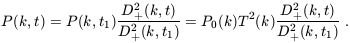
3.2. The Galaxy Power-spectrum

Although the traditional tool for studying galaxy clustering is the two-point correlation function, (r) [Peebles 1980], defined by

(23)

the (small) joint probability of finding two galaxies in the (small) volumes dV₁ and dV₂ separated by a distance r when the mean number-density of galaxies is n. Most modern analyses concentrate instead upon its Fourier transform, the power-spectrum P(k). This is especially useful because it is the power-spectrum which is predicted directly in cosmogonical models incorporating inflation and dark matter. For example, Peacock & Dodds have recently made compilations of power-spectra of different kinds of galaxy and cluster redshift samples and, for comparison, a deprojection of the APM w() [Peacock & Dodds 1996]. Within the (considerable) observational errors, and the uncertainty introduced by modelling of the bias, all the data lie roughly on the same curve. A consistent picture thus seems to have emerged in which galaxy clustering extends over larger scales than is expected in the standard CDM scenario. Considerable uncertainty nevertheless remains about the shape of the power spectrum on very large scales.

3.3. The abundances of objects

In addition to their spatial distribution, the number-densities of various classes of cosmic objects as a function of redshift can be used to constrain the shape of the power-spectrum. In particular, if objects are forming by hierarchical merging there should be fewer objects of a given mass at high z and more objects with lower mass. This can be made quantitative fairly simply, using an analytic method [Press & Schechter 1974]. Although this kind of argument can be applied to many classes of object [Ma et al. 1997], it potentially yields the strongest constraints when applied to galaxy clusters. At the moment, results are controversial, but the evolution of cluster numbers with redshift is such sensitive probe of so that future studies of high-redshift clusters may yield more definitive results [Eke et al. 1996, Blanchard et al. 1999].

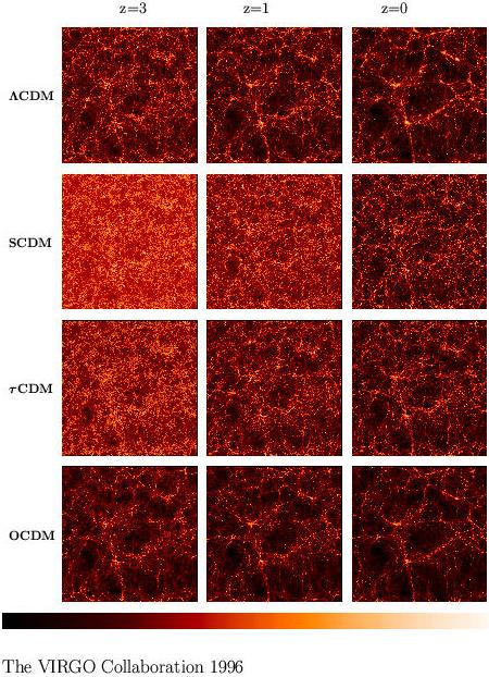
3.4. High-redshift clustering

It is evident from Figure 1 that, although the three non-SCDM models are similar at z = 0, differences between them are marked at higher redshift. This suggests the possibility of using measurements of galaxy clustering at high redshift to distinguish between models and reality. This has now become possible, with surveys of galaxies at z ~ 3 already being constructed [Steidel et al. 1998]. Unfortunately, the interpretation of these new data is less straightforward than one might have imagined. If the galaxy distribution is biased at z = 0 then the bias is expected to grow with z [Davis et al. 1985]. If galaxies are rare peaks now, they should have been even rarer at high z. There are also many distinct possibilities as to how the bias might evolve with redshift [Moscardini et al. 1998]. Theoretical uncertainties therefore make it difficult to place stringent constrains on models, although with more data and better theoretical modelling, high-redshift clustering measurements will play a very important role in forthcoming years.

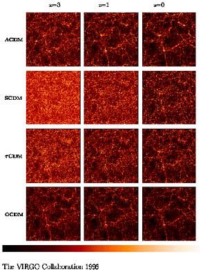
Figure 1. Some of the candidate models described in the text, as simulated by the Virgo consortium. Notice that SCDM shows very different structure at z = 0 than the three alternatives shown. The models also differ significantly at different epochs. These simulat ions show the distribution of dark matter only.

3.5. Higher-order Statistics

The galaxy power-spectrum has rightly played a central role in the development of this subject, but the information it contains is in fact rather limited. In more precise terms, it is called a second-order statistic as it contains information equivalent to the second moment (i.e. variance) of a random variable. Higher-order statistics would be necessary to provide a complete statistical description of clustering pattern and these generally require large, well-sampled data sets [Sahni & Coles 1985]. One particularly promising set of descriptors emerge from the realisation [Coles & Frenk 1991, Bernardeau 1994, Colombi et al. 1996] that higher-order moments grow by gravitational instability in a manner that couples directly to the growth of the variance. This offers the prospect of being able to distinguish between genuine clustering produced by gravity and clustering induced by bias.

3.6. Peculiar Motions

There are various ways in which it is possible to use information about the velocities of galaxies to constrain models [Strauss & Willick 1995]. Probably the most useful information pertains to large-scale motions, as small-scale data populate the highly nonlinear regime.

The basic principle is that velocities are induced by fluctuations in the total mass, not just the galaxies. Comparing measured velocities with measured fluctuations in galaxies with measured fluctuations in galaxy counts, it is possible to constrain both and b. From equations (11)-(13) it emerges that

(24)

which demonstrates that the velocity flow associated with the growing mode in the linear regime is curl-free, as it can be expressed as the gradient of a scalar potential function. Notice also that the induced velocity depends on . This is the basis of a method for estimating which is known as POTENT [Dekel 1994]. Since all matter gravitates, not just the luminous material, there is a hope that methods such as this can break the degeneracy between clustering induced by gravity and that induced statistically, by bias.

These methods are prone to error if there are errors in the velocity estimates. Perhaps a more robust approach is to use peculiar motion information indirectly, by the effect they have on the distribution of galaxies seen in redshift-space (i.e. assuming total velocity is proportional to distance). The information gained this way is statistical, but less prone to systematic error [Heavens & Taylor 1995].

3.7. Gravitational Lensing

Another class of observations that can help break the degeneracy between models involves gravitational lensing. The most spectacular forms of lensing are those producing multiple images or strong distortions in the form of arcs. These require very large concentrations of mass and are therefore not so useful for mapping the structure on large scales. However, there are lensing effects that are much weaker than the formation of multiple images. In particular, distortions producing a shearing of galaxy images promise much in this regard [Kaiser & Squires 1993]. With the advent of new large CCD detectors, this should soon be realised [Mellier 1999], although present constraints are quiet weak.

3.8. The Cosmic Microwave Background

I have so far avoided discussion of the cosmic microwave background, but this probably holds the key to unlocking many of the present difficulties in large-scale structure models. Although the COBE data [Smoot et al. 1992] do not constrain the shape of the matter power spectrum on scales of direct relevance to structures we can see in the galaxy distribution, finer-scale maps will do so in the near future. ESA's Planck Explorer and NASA's MAP experiment will measure the properties of matter fluctuations in the linear without having to worry about the confusion caused by non-linearity and bias when galaxy counts are used. It is hoped that measurements of particular features in the angular power-spectrum of the fluctuations [Hu & Sugiyama 1995] measured by these experiments will pin down the densities of CDM, HDM, baryons and vacuum energy (i.e. ) as well as fixing and H. Experiments such as BOOMERANG and MAXIMA are already leading to interesting results, but these are discussed elsewhere in this volume.

4. TESTING COSMOLOGICAL GAUSSIANITY

Largely motivated by the idea that they were generated by quantum fluctuations during a period of inflation, most fashionable models of structure formation involve the assumption that the initial fluctuations constitute a Gaussian random field. Mathematically, this assumption means that all finite- dimensional joint probability distributions of the density at different spatial locations can be expressed as multivariate normal distributions. This is much stronger than the assertion that the distribution of densities should be a normal distribution. It is quite possible for a field to have a Gaussian one-point probability distribution but be non-Gaussian in the sense used here. Testing this form of multivariate normality in an arbitrary number of dimensions is a decidedly non-trivial task, but is necessary given the importance of the assumption. If it can be shown that the large-scale structure of the Universe is inconsistent with Gaussian initial data this will have profound implications for fundamental physics. This issue does not therefore represent a mere exercise in statistics, but a vital step towards a physical understanding of the origin and evolution of the large-scale structure of the Universe.

As well as being physically motivated, the Gaussian assumption has great advantage that it is a mathematically complete prescription for all the statistical properties of the initial density field, once the fluctuation amplitude is specified as a function of scale through the power-spectrum P(k). In Fourier terms, a Gaussian random field consists of a stochastic superposition of plane waves. The amplitude of each mode, A_k, is drawn from a distribution specified by the power-spectrum and its phase, _k, is uniformly random and independent of the phases of all other modes. As the fluctuations evolve in time, the density distribution becomes non-Gaussian. But this departure from non-Gaussianity depends on gravity being able to move material from its primordial position. On scales much larger than the typical scale of such motions, the distribution remains Gaussian. The distribution of matter today should therefore be highly non-Gaussian on small scales, gradually tending closer to Gaussian on progressively larger scales. Any non-Gaussianity detected at the present epoch could therefore either be primordial, or produced dynamically, or could could be imposed by variations in mass-to-light ratio (bias), or all of these. Galaxy clustering statistics therefore need to be devised that can separate these different signatures.

The distribution of temperature fluctuations in the cosmic microwave background (CMB), which was imprinted before significant gravitational evolution took place, should also retain the character of the initial statistics. Any non-Gaussianity detected here could either be primordial, produced by errors in foreground subtraction or other systematics. Again, tests capable of distinguishing between these possibilities are required.

Gaussian models have generally fared much better in comparison with data than others with non-Gaussian initial data, such as those based on topological defects, although predictions in the second category of models are harder to come by because of the much greater calculational difficulties involved. It is fair to say, however, that as far as existing data are concerned the large-scale distribution of mass certainly seems to be consistent with Gaussian statistics. Initially, it also appeared that the COBE fluctuations in temperature of the CMB were also consistent with Gaussian primordial perturbations. On the other hand, the statistical descriptors necessary to carry out a powerful test against the Gaussian require much higher quality data than has so far been furnished by galaxy surveys. Moreover, the non-Gaussianity induced by gravitational evolution, redshift-space effects, and variations in mass-to-light ratio has complicated the interpretation of the data, although recent theoretical developments discussed below should ameliorate these problems.

In the following I discuss a method of quantifying phase information [Chiang & Coles 2000] and suggest how this information may be exploited to build novel statistical descriptors that can be used to mine the sky more effectively than with standard methods.

4.1. Fourier Description of Cosmological Density Fields

In most popular versions of the ``gravitational instability'' model for the origin of cosmic structure, particularly those involving cosmic inflation [Guth & Pi 1982], the initial fluctuations that seeded the structure formation process form a Gaussian random field [Bardeen et al. 1986]. Because the initial perturbations evolve linearly, it is useful to expand (x) as a Fourier superposition of plane waves:

(25)

The Fourier transform (k) is complex and therefore possesses both amplitude |(k)| and phase _k where

(26)

Gaussian random fields possess Fourier modes whose real and imaginary parts are independently distributed. In other words, they have phase angles _k that are independently distributed and uniformly random on the interval [0, 2]. When fluctuations are small, i.e. during the linear regime, the Fourier modes evolve independently and their phases remain random. In the later stages of evolution, however, wave modes begin to couple together [Peebles 1980]. In this regime the phases become non-random and the density field becomes highly non-Gaussian. Phase coupling is therefore a key consequence of nonlinear gravitational processes if the initial conditions are Gaussian and a potentially powerful signature to exploit in statistical tests of this class of models.

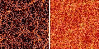
A graphic demonstration of the importance of phases in patterns generally is given in Fig 2. Since the amplitude of each Fourier mode is unchanged in the phase reshuffling operation, these two pictures have exactly the same power-spectrum, P(k) |(k)|². In fact, they have more than that: they have exactly the same amplitudes for all k. They also have totally different morphology. Further demonstrations of the importance of Fourier phases in defining clustering morphology are given by Chiang (2001). The evident shortcomings of P(k) can be partly ameliorated by defining higher-order quantities such as the bispectrum [Peebles 1980, Matarrese et al. 1997, Scoccimarro et al. 1999, Verde et al. 2000] or correlations of (k)² [Stirling & Peacock 1996].

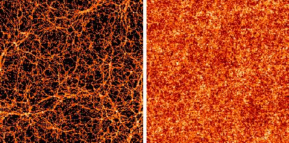
Figure 2. Numerical simulation of galaxy clustering (left) together with a version generated randomly reshuffling the phases between Fourier modes of the original picture (right).

4.2. The Bispectrum and Phase Coupling

The bispectrum and higher-order polyspectra vanish for Gaussian fields, but in a non-Gaussian field they may be non-zero. The usefulness of these and related quantities therefore lies in the fact that they encode some information about non-linearity and non-Gaussianity. To understand the relationship between the bispectrum and Fourier phases, it is very helpful to consider the following toy examples. Imagine a simple density field defined in one spatial dimension that consists of the superposition of two cosine components:

(27)

The generalisation to several spatial dimensions is trivial. The phases ₁ and ₂ are random and A₁ and A₂ are constants. We can simplify the following by introducing a new notation

(28)

Clearly this example displays no phase correlations. Now consider a new field obtained from the example (27) through the non-linear transformation

(29)

where is a constant parameter. Equation (29) may be thought of as a very phenomenological representation of a perturbation series, with controlling the level of non-linearity. Using the same notation as equation (28), the new field (x) can be written

(30)

where the B_i are constants obtained from the A_i. Notice in equation (30) that the phases follow the same kind of harmonic relationship as the wavenumbers. This form of phase association is termed quadratic phase coupling. It is this form of phase relationship that appears in the bispectrum. To see this, consider another two toy examples. First, model A,

(31)

in which ₃ = ₁ + ₂ but in which ₁, ₂ and ₃ are random; and

(32)

Model A exhibits no phase association; model B displays quadratic phase coupling. It is straightforward to show that < _A > = < _B > = 0. The autocovariances are equal:

(33)

as are the power spectra, demonstrating that second-order statistics are blind to phase association. The (reduced) three-point autocovariance function is

(34)

For model A we get

(35)

whereas for model B it is

(36)

The bispectrum, B(k₁, k₂), is defined as the two-dimensional Fourier transform of , so B_A(k₁, k₂) = 0 trivially, whereas B_B(k₁, k₂) consists of a single spike located somewhere in the region of (k₁, k₂) space defined by k₂ 0, k₁ k₂ and k₁ + k₂ . If _{1 2} then the spike appears at k₁ = ₁, k₂ = ₂). Thus the bispectrum measures the phase coupling induced by quadratic nonlinearities. To reinstate the phase information order-by-order requires an infinite hierarchy of polyspectra.

An alternative way of looking at this issue is to note that the information needed to fully specify a non-Gaussian field to arbitrary order (or, in a wider context, the information needed to define an image resides in the complete set of Fourier phases [Oppenheim & Lim 1981]. Unfortunately, relatively little is known about the behaviour of Fourier phases in the nonlinear regime of gravitational clustering [Ryden & Gramman 1991, Scherrer et al. 1991, Soda & Suto 1992, Jain & Bertschinger 1996, Jain & Bertschinger 1998, Coles & Chiang 2000], but it is of great importance to understand phase correlations in order to design efficient statistical tools for the analysis of clustering data.

4.3. Visualizing and Quantifying Phase Information

A vital first step on the road to a useful quantitative description of phase information is to represent it visually [Coles & Chiang 2000]. In colour image display devices, each pixel represents the intensity and colour at that position in the image [Thornton 1998, Foley & Van Dam 1982]. The quantitative specification of colour involves three coordinates describing the location of that pixel in an abstract colour space, designed to reflect as accurately as possible the eye's response to light of different wavelengths. In many devices this colour space is defined in terms of the amount of Red, Green or Blue required to construct the appropriate tone; hence the RGB colour scheme. The scheme we are particularly interested in is based on three different parameters: Hue, Saturation and Brightness. Hue is the term used to distinguish between different basic colours (blue, yellow, red and so on). Saturation refers to the purity of the colour, defined by how much white is mixed with it. A saturated red hue would be a very bright red, whereas a less saturated red would be pink. Brightness indicates the overall intensity of the pixel on a grey scale. The HSB colour model is particularly useful because of the properties of the `hue' parameter, which is defined as a circular variable. If the Fourier transform of a density map has real part R and imaginary part I then the phase for each wavenumber, given by = arctan(I / R), can be represented as a hue for that pixel using the colour circle [Coles & Chiang 2000].

The pattern of phase information revealed by this method related to the gravitational dynamics of its origin. For example in our analysis of phase coupling [Chiang & Coles 2000] we introduced a quantity D_k, defined by

(37)

which measures the difference in phase of modes with neighbouring wavenumbers in one dimension. We refer to D_k as the phase gradient. To apply this idea to a two-dimensional simulation we simply calculate gradients in the x and y directions independently. Since the difference between two circular random variables is itself a circular random variable, the distribution of D_k should initially be uniform. As the fluctuations evolve waves begin to collapse, spawning higher-frequency modes in phase with the original [Shandarin & Zel'dovich 1989]. These then interact with other waves to produce a non-uniform distribution of D_k. For examples, see

http://www.nottingham.ac.uk/~ppzpc/phases/index.html.

It is necessary to develop quantitative measures of phase information that can describe the structure displayed in the colour representations. In the beginning the phases _k are random and so are the D_k obtained from them. This corresponds to a state of minimal information, or in other words maximum entropy. As information flows into the phases the information content must increase and the entropy decrease. One way to quantify this is by defining an information entropy on the set of phase gradients. One constructs a frequency distribution, f (D) of the values of D_k obtained from the whole map. The entropy is then defined as

(38)

where the integral is taken over all values of D, i.e. from 0 to 2. The use of D, rather than itself, to define entropy is one way of accounting for the lack of translation invariance of , a problem that was missed in previous attempts to quantify phase entropy [Polygiannikis & Moussas 1995]. A uniform distribution of D is a state of maximum entropy (minimum information), corresponding to Gaussian initial conditions (random phases). This maximal value of S_max = log(2) is a characteristic of Gaussian fields. As the system evolves it moves into to states of greater information content (i.e. lower entropy). The scaling of S with clustering growth displays interesting properties [Chiang & Coles 2000], establishing an important link between the spatial pattern and the physics driving clustering growth.

5. BIAS AND HIERARCHICAL CLUSTERING

The biggest stumbling-block for attempts to confront theories of cosmological structure formation with observations of galaxy clustering is the uncertain and possibly biased relationship between galaxies and the distribution of gravitating matter. The idea that galaxy formation might be biased goes back to the realization by Kaiser (1984) that the reason Abell clusters display stronger correlations than galaxies at a given separation is that these objects are selected to be particularly dense concentrations of matter. As such, they are very rare events, occurring in the tail of the distribution function of density fluctuations. Under such conditions a ``high-peak'' bias prevails: rare high peaks are much more strongly clustered than more typical fluctuations (Bardeen et al. 1986). If the properties of a galaxy (its morphology, color, luminosity) are influenced by the density of its parent halo, for example, then differently-selected galaxies are expected to a different bias (e.g. Dekel & Rees 1987). Observations show that different kinds of galaxy do cluster in different ways (e.g. Loveday et al. 1995; Hermit et al. 1996).

In local bias models, the propensity of a galaxy to form at a point where the total (local) density of matter is is taken to be some function f () (Coles 1993, hereafter C93; Fry & Gaztanaga 1993, hereafter FG93). It is possible to place stringent constraints on the effect this kind of bias can have on galaxy clustering statistics without making any particular assumption about the form of f. In this Letter, we describe the results of a different approach to local bias models that exploits new results from the theory of hierarchical clustering in order to place stronger constraints on what a local bias can do to galaxy clustering. We leave the technical details to Munshi et al. (1999a, b) and Bernardeau & Schaeffer (1999); here we shall simply motivate and present the results and explain their importance in a wider context.

5.1. Hierarchical Clustering

The fact that Newtonian gravity is scale-free suggests that the N-point correlation functions of self-gravitating particles, _N, evolved into the large-fluctuation regime by the action of gravity, should obey a scaling relation of the form

(39)

when the elements of a structure are scaled by a factor (e.g. Balian & Schaeffer 1989). Observations offer some support for such an idea, in that the observed two-point correlation function (r) of galaxies is reasonably well represented by a power law over a large range of length scales,

(40)

(Groth & Peebles 1977; Davis & Peebles 1977) for r between, say, 100h^-1 kpc and 10h^-1 Mpc. The observed three point function, ₃, is well-established to have a hierarchical form

(41)

where _ab = (x_a, x_b), etc, and Q is a constant (Davis & Peebles 1977; Groth & Peebles 1977). The four-point correlation function can be expressed as a combination of graphs with two different topologies - ``snake'' and ``star'' - with corresponding (constant) amplitudes R_a and R_b respectively:

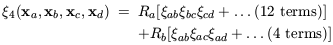
(42)

(e.g. Fry & Peebles 1978; Fry 1984).

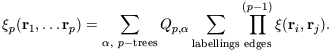
It is natural to guess that all p-point correlation functions can be expressed as a sum over all possible p-tree graphs with (in general) different amplitudes Q_p, for each tree diagram topology . If it is further assumed that there is no dependence of these amplitudes upon the shape of the diagram, rather than its topology, the correlation functions should obey the following relation:

(43)

To go further it is necessary to find a way of calculating Q_p. One possibility, which appears remarkably successful when compared with numerical experiments (Munshi et al. 1999b; Bernardeau & Schaeffer 1999), is to calculate the amplitude for a given graph by simply assigning a weight to each vertex of the diagram _n, where n is the order of the vertex (the number of lines that come out of it), regardless of the topology of the diagram in which it occurs. In this case

(44)

Averages of higher-order correlation functions can be defined as

(45)

Higher-order statistical properties of galaxy counts are often described in terms of the scaling parameters S_p constructed from the _p via

(46)

It is a consequence of the particular class of hierarchical clustering models defined by equations (5) & (6) that all the S_p should be constant, independent of scale.

5.2. Local Bias

Using a generating function technique [Bernardeau & Schaeffer 1992] it is possible to derive a series expansion for the m-point count probability distribution function of the objects P_m(N₁, .... N_m) (the joint probability of finding N_i objects in the i-th cell, where i runs from 1 to m) from the _n. The hierarchical model outlined above is therefore statistically complete. In principle, therefore, any statistical property of the evolved distribution of matter can be calculated just as it can for a Gaussian random field. This allows us to extend various results concerning the effects of biasing on the initial conditions into the nonlinear regime in a more elegant way than is possible using other approaches to hierarchical clustering.

For example, let us consider the joint probability P₂(N₁, N₂) for two cells to contain N₁ and N₂ particles respectively. Using the generating-function approach outlined above, it is quite easy to show that, at lowest order,

(47)

where the P₁(N_i) are the individual count probabilities of each volume separately and ₁₂ is the underlying mass correlation function. The function b(N_i) we have introduced in (9) depends on the set of _n appearing in equation (6); its precise form does not matter in this context, but the structure of equation (9) is very useful. We can use (9) to define

(48)

where _N1N2(r₁₂) is the cross-correlation of ``cells'' of occupancy N₁ and N₂ respectively. From this definition and equation (9) it follows that

(49)

we have dropped the subscripts on r for clarity from now on. From (11) we can obtain

(50)

for the special case where N₁ = N₂ = N which can be identified with the usual definition of the bias parameter associated with the correlations among a given set of objects _obj(r) = b²_{obj mass}(r). Moreover, note that at this order (which is valid on large scales), the correlation bias defined by equation (11) factorizes into contributions b_Ni from each individual cell (Bernardeau 1996; Munshi et al. 1999b).

Coles (1993) proved, under weak conditions on the form of a local bias f () as discussed in the introduction, that the large-scale biased correlation function would generally have a leading order term proportional to ₁₂(r₁₂). In other words, one cannot change the large-scale slope of the correlation function of locally-biased galaxies with respect to that of the mass. This ``theorem'' was proved for bias applied to Gaussian fluctuations only and therefore does not obviously apply to galaxy clustering, since even on large scales deviations from Gaussian behaviour are significant. It also has a more minor loophole, which is that for certain peculiar forms of f the leading order term is proportional to ₁₂², which falls off more sharply than ₁₂ on large scales.

Steps towards the plugging of this gap began with FG93 who used an expansion of f in powers of and weakly non-linear (perturbative) calculations of ₁₂(r) to explore the statistical consequences of biasing in more realistic (i.e. non-Gaussian) fields. Based largely on these arguments, Scherrer & Weinberg (1998), hereafter SW98, confirmed the validity of the C93 result in the non-linear regime, and also showed explicitly that non-linear evolution always guarantees the existence of a linear leading-order term regardless of f, thus plugging the small gap in the original C93 argument. These works have a similar motivation the approach I am discussing here, and also exploit hierarchical scaling arguments of the type discussed above en route to their conclusions. What is different about the approach we have used in this paper is that the somewhat cumbersome simultaneous expansion of f and ₁₂ used by SW98 is not required in this calculation. The generating functions to proceed directly to the joint probability (9), while SW98 have to perform a complicated sum over moments of a bivariate distribution. The factorization of the probability distribution (9) is also a stronger result than that presented by SW98, in that it leads almost trivially to the C93 ``theorem'' but also generalizes to higher-order correlations than the two-point case under discussion here.

Note that the density of a cell of given volume is simply proportional to its occupation number N. The factorizability of the dependence of _N1N2(r₁₂) upon b(N₁) and b(N₂) in (11) means that applying a local bias f () boils down to applying some bias function F(N) = f[b(N)] to each cell. Integrating over all N thus leads directly to the same conclusion as C93, i.e. that the large-scale (r) of locally-biased objects is proportional to the underlying matter correlation function. This has also been confirmed by numerically using N-body experiments (Mann et al. 1998; Narayanan et al. 1998).

5.3. Halo Bias

In hierarchical models, galaxy formation involves the following three stages:

1. the formation of a dark matter halo;

2. the settling of gas into the halo potential;

3. the cooling and fragmentation of this gas into stars.

Rather than attempting to model these stages in one go by a simple function f of the underlying density field it is interesting to see how each of these selections might influence the resulting statistical properties. Bardeen et al. (1986), inspired by Kaiser (1984), pioneered this approach by calculating detailed statistical properties of high-density regions in Gaussian fluctuations fields. Mo & White (1996) and Mo et al. (1997) went further along this road by using an extension of the Press-Schechter (1974) theory to calculate the correlation bias of halos, thus making an attempt to correct for the dynamical evolution absent in the Bardeen et al. approach. The extended Press-Schechter approach seem to be in good agreement with numerical simulations, except for small halo masses (Jing 1998). It forms the basis of many models for halo bias in the subsequent literature (e.g. Moscardini et al. 1998; Tegmark & Peebles 1998).

The hierarchical models furnish an elegant extension of this work that incorporates both density-selection and non-linear dynamics in an alternative to the Mo & White (1996) approach. We exploit the properties of equation (47) to construct the correlation function of volumes where the occupation number exceeds some critical value. For very high occupations these volumes should be in good correspondence with collapsed objects.

The way of proceeding is to construct a tree graph for all the points in both volumes. One then has to re-partition the elements of this graph into internal lines (representing the correlations within each cell) and external lines (representing inter-cell correlations). Using this approach the distribution of high-density regions in a field whose correlations are given by eq. (5) can be shown to be itself described by a hierarchical model, but one in which the vertex weights, say M_n, are different from the underlying weights _n (Bernardeau & Schaeffer 1992, 1999; Munshi et al. 1999a, b).

First note that a density threshold is in fact a form of local bias, so the effects of halo bias are governed by the same strictures as described in the previous section. Many of the other statistical properties of the distribution of dense regions can be reduced to a dependence on a scaling parameter x, where

(51)

In this definition N_c = ₂, where is the mean number of objects in the cell and ₂ is defined by eq. (45) with p = 2. The scaling parameters S_p can be calculated as functions of x, but are generally rather messy (Munshi et al. 1999a). The most interesting limit when x >> 1 is, however, rather simple. This is because the vertex weights describing the distribution of halos depend only on the _n and this dependence cancels in the ratio (46). In this regime,

(52)

for all possible hierarchical models. The reader is referred to Munshi et al. (1999a) for details. This result is also obtained in the corresponding limit for very massive halos by Mo et al. (1997). The agreement between these two very different calculations supports the inference that this is a robust prediction for the bias inherent in dense regions of a distribution of objects undergoing gravity-driven hierarchical clustering.

5.4. Progress on Biasing

The main purpose of this lecture has been to discuss recent developments in the theory of gravitational-driven hierarchical clustering. The model described in equations (5) & (6) provides a statistically-complete prescription for a density field that has undergone hierarchical clustering. This allows us to improve considerably upon biasing arguments based on an underlying Gaussian field.

These methods allow a simpler proof of the result obtained by SW98 that strong non-linear evolution does not invalidate the local bias theorem of C93. They also imply that the effect of bias on a hierarchical density field is factorizable. A special case of this is the bias induced by selecting regions above a density threshold. The separability of bias predicted in this kind of model could be put to the test if a population of objects could be found whose observed characteristics (luminosity, morphology, etc.) were known to be in one-to-one correspondence with the halo mass. Likewise, the generic prediction of higher-order correlation behaviour described by the behaviour of S_p in equation (46) can also be used to construct a test of this particular form of bias.

Referring to the three stages of galaxy formation described in § 4, analytic theory has now developed to the point where it is fairly convincing on (1) the formation of halos. Numerical experiments are beginning now to handle (2) the behaviour of the gas component (Blanton et al. 1998, 1999). But it is unlikely that much will be learned about (3) by theoretical arguments in the near future as the physics involved is poorly understood (though see Benson et al. 1999). Arguments have already been advanced to suggest that bias might not be a deterministic function of , perhaps because of stochastic or other hidden effects (Dekel & Lahav 1998; Tegmark & Bromley 1999). It also remains possible that large-scale non-local bias might be induced by environmental effects (Babul & White 1991; Bower et al. 1993).

Before adopting these more complex models, however, it is important to exclude the simplest ones, or at least deal with that part of the bias that is attributable to known physics. At this stage this means that the `minimal' bias model should be that based on the selection of dark matter halos. Establishing the extent to which observed galaxy biases can be explained in this minimal way is clearly an important task.

6. DISCUSSION

In fairly recent history, cosmological data sets were sparse and incomplete, and the statistical methods deployed to analyse them were crude. Second-order statistics, such as P(k) and (r), are blunt instruments that throw away the fine details of the delicate pattern of cosmic structure. These details lie in the distribution of Fourier phases to which second-order statistics are blind. It would not do justice to massively improved data if effort were directed only to better estimates of these quantities. Moreover, as we have shown, phase information provides a unique fingerprint of gravitational instability developed from Gaussian initial conditions (which have maximal phase entropy). Methods such as those described above can therefore be used to test this standard paradigm for structure formation. They can also furnish direct tests of the presence of initial non-Gaussianity [Ferreira et al. 1998, Pando et al. 1998, Bromley & Tegmark 1999].

But there is also an important general point to be made about the philosophy of large-scale structure studies. The existing approaches are dominated by a direct methodology. A hypothetical mixture of ingredients is constructed (see Section 2.6), and ab initio simulations used to propagate the initial conditions to a model of reality that would pertain if the model were true. If it fails, one revises the model. But there are now many models which agree more-or-less with the existing data. These also contain free parameters that can be used to massage them into compliance with observations. In particular, we can appeal to a complex non-linear and non-local bias to achieve this. The usefulness of these direct hypothesis tests is therefore open to doubt.

The stumbling block lies with the fact that we still cannot reliably predict the relationship between galaxies and mass. Although theory seems to have slowed down, we do now have the prospect of huge amounts of data arriving on the scene. A better approach than the direct one I have mentioned is to treat those unknown aspects of galaxy formation as an inverse problem. Given a sufficiently flexible and realistic model we should infer parameter values from observations. To exploit this approach requires the development of simple models that can be used to close the inductive loop connecting theory with observations. For this reason it is important to continue constructing simple models of bias and galaxy clustering generally, since these are such valuable inferential tools.

As the raw material is increasing in both quality and quantity, it is time to refine our statistical technology so that the subtle and precious artifacts previously ignored can be both detected and extracted.

REFERENCES

1. P.P. Avelino, E.P.S. Shellard, J.H.P. Wu, & B. Allen, ApJ, 507 (1998), L101
2. A. Babul & S.D.M. White, MNRAS, 253 (1991), L31
3. J.M. Bardeen, J.R. Bond, N. Kaiser & A.S. Szalay, ApJ, 304 (1986), 15
4. C.M. Baugh, S. Cole, C.S. Frenk, C.G. Lacey, ApJ, 498 (1998), 504
5. A.J. Benson, S. Cole, C.S. Frenk, C.M. Baugh & C.G. Lacey, 1999, MNRAS, submitted, astro-ph/9903343
6. F. Bernardeau, ApJ, 433 (1994), 1
7. F. Bernardeau, A& A, 312 (1996), 11
8. F. Bernardeau & R. Schaeffer, A& A, 255 (1992), 1
9. F. Bernardeau & R. Schaeffer, A& A, 349 (1999), 697
10. A. Blanchard, R. Sadat, J.G. Barlett & M. Le Dour, A& A, submitted, astro-ph/9908037 (1999)
11. M. Blanton, R. Cen, J.P. Ostriker & M.A. Strauss, 1998, ApJ, submitted, astro-ph/9807029
12. M. Blanton, R. Cen, J.P. Ostriker, M.A. Strauss & M. Tegmark, 1999, ApJ, submitted, astro-ph/9903165
13. R.G. Bower, P. Coles, C.S. Frenk & S.D.M. White, ApJ, 405 (1993), 403
14. R.H. Brandenberger, Rev. Mod. Phys., 57 (1985), 1
15. B.C. Bromley & M. Tegmark, ApJ, 524 (1999), L79
16. R. Cen, ApJS, 78 (1992), 341
17. L.-Y. Chiang & P. Coles, MNRAS, 311 (2000), 809
18. L.-Y. Chiang, MNRAS, in press, astro-ph/0011021 (2001)
19. P. Coles, MNRAS, 262 (1993), 1065
20. P. Coles & L.-Y. Chiang, Nature, 406 (2000), 376
21. P. Coles & C.S. Frenk, MNRAS, 253 (1991), 727
22. P. Coles, A.L. Melott & D. Munshi, ApJ, 521 (1999), L5
23. P. Coles et al., MNRAS, 264 (1993), 749
24. M. Colless, preprint, astro-ph/9804079 (1998)
25. S. Colombi, F.R. Bouchet & L. Hernquist, ApJ, 465 (1996), 14
26. M. Davis, G. Efstathiou, C.S. Frenk & S.D.M. White, ApJ, 292 (1985), 371
27. M. Davis & P.J.E. Peebles, ApJS, 34 (1977), 425
28. A. Dekel, ARA& A, 32 (1994), 371
29. A. Dekel & O. Lahav, O., 1998, preprint, astro-ph/9806193
30. A. Dekel & M.J. Rees, Nature, 326 (1987), 455
31. A. Dekel & O. Lahav, ApJ, 520 (1999), 24
32. V. de Lapparent, M.J. Geller & J.P. Huchra, ApJ, 302 (186), L1
33. G. Efstathiou, W.J. Sutherland, S.J. Maddox, Nature, 348 (1990), 705
34. V.R. Eke, S. Cole & C.S. Frenk, MNRAS, 282 (1996), 263
35. P.G. Ferreira, J. Magueijo & K.M. Górski, ApJ, 503 (1998), L1
36. J.D. Foley & A. Van Dam, Fundamentals of Interactive Computer Graphics. Addison-Wesley, Reading, Mass., (1982)
37. J.N. Fry, ApJ, 279 (19884), 499
38. J.N. Fry & E. Gaztanaga, ApJ, 413 (1993), 447
39. J.N. Fry & P.J.E. Peebles, 1978, ApJ, 221 (1978), 19
40. S. Gottlöber, J.P. Mucket & A.A. Starobinsky, ApJ, 434 (1994), 417
41. E. Groth & P.J.E. Peebles, ApJ, 217 (1977), 385
42. J.E. Gunn & D.H. Weinberg, in: Wide Field Spectroscopy and ther Distant Universe, eds. S.J. Maddox & A. Aragón-Salamanca, World Scientific, Singapore, pp. 3-14 (1995)
43. A.H. Guth, Phys. Rev. D., 23 (1981), 347
44. A.H. Guth & S.-Y. Pi Phys. Rev. Lett., 49 (1982), 1110
45. E.R. Harrison, Phys. Rev. D., 1 (1970), 2726
46. A.F. Heavens & A.N. Taylor, MNRAS, 275 (1995), 483
47. S. Hermit et al., MNRAS, 283 (1996), 709
48. W. Hu & N. Sugiyama, Phys. Rev. D, 51 (1995), 2599
49. B. Jain & E. Bertschinger, ApJ, 456 (1996), 43
50. B. Jain & E. Bertschinger, ApJ, 509 (1998), 517P
51. A. Jenkins et al., ApJ, 499 (1998), 20
52. N. Kaiser, ApJ, 284 (1984), L9
53. N. Kaiser & G. Squires, ApJ, 404 (1993), 441
54. A. Klypin, J.A. Holtzmann, J. Primack & E. Regos, ApJ, 416 (1993), 1
55. J.E. Lidsey & P. Coles, MNRAS, 258 (1992), 57P
56. J. Loveday, S.J. Maddox, G. Efstathiou, B.A. Peterson, ApJ, 442 (1995), 457
57. C. Ma, E. Bertschinger, L. Hernquist, D.H. Weinberg & N. Katz, ApJ, 484 (1997), L1
58. R.G. Mann, J.A. Peacock & A.F. Heavens, MNRAS, 293 (1998), 209
59. S. Matarrese, L. Verde & A.F. Heavens, MNRAS 290 (1997), 651
60. Y. Mellier, ARA& A, in press, astro-ph/9812172 (1999)
61. H.-J. Mo & S.D.M. White, MNRAS, 282 (1996), 347
62. H.-J. Mo, Y.-P. Jing & S.D.M. White, MNRAS, 284 (1997), 189
63. L. Moscardini, P. Coles, F. Lucchin & S. Matarrese, MNRAS, 299 (1998), 95
64. D. Munshi, P. Coles & A.L. Melott, MNRAS, 307 (1999a), 387
65. D. Munshi, P. Coles & A.L. Melott, MNRAS, 310 (1999b), 892
66. V.K. Narayanan, A.A. Berlind, & D.H. Weinberg, 1998, preprint, astro-ph/9812002
67. A.V. Oppenheim & J.S. Lim, Proc. IEEE. 69 (1981), 529
68. J. Pando, D. Valls-Gabaud & L.-Z. Fang, Phys. Rev. Lett., 81 (1998), 4568
69. J.A. Peacock & S.J. Dodds, MNRAS, 280 (1996), L19
70. P.J.E. Peebles, The Large-scale Structure of the Universe (Princeton University Press, Princeton, 1980)
71. P.J.E. Peebles, ApJ, 510 (1999), 523
72. P.J.E. Peebles, ApJ, 510 (1999), 531
73. S. Perlmutter et al., ApJ, 517 (1999), 565
74. E. Pierpaoli, P. Coles, S. Bonometto & S. Borgani, ApJ, 470 (1996), 92
75. J.M. Polygiannikis & X. Moussas, Solar Physics, 158 (1995), 159
76. W.H. Press & P. Schechter, ApJ, 187 (1974), 425
77. B.S. Ryden & M. Gramann, ApJ, 383 (1991), L33
78. V. Sahni & P. Coles, Phys. Rep., 262 (1995), 1
79. R.J. Scherrer, A.L. Melott & S.F Shandarin, ApJ, 377 (1991), 29
80. R.J. Scherrer & D.H. Weinberg, ApJ, 504 (1998), 607
81. R. Scoccimarro, H.M.P. Couchman & J. Frieman, ApJ, 517 (1999), 531
82. S.F. Shandarin & Ya. B. Zel'dovich, Rev. Mod. Phys., 61 (1989), 185
83. S.A. Shectman et al., ApJ, 1996, ApJ, 470 (1996), 172
84. G.F. Smoot et al., ApJ, 396 (1992), L1
85. J. Soda & Y. Suto, ApJ, 396 (1992), 379
86. C.C. Steidel et al., ApJ, 492 (1998), 428
87. A.J. Stirling & J.A. Peacock, MNRAS, 283 (1996), L99
88. M.A. Strauss & J.A. Willick, Phys. Rep., 261 (1995), 271
89. M. Tegmark & B.C. Bromley, ApJ, 518 (1999), L69
90. M. Tegmark & P.J.E. Peebles, ApJ, 500 (1998), L79
91. A.L. Thornton, Colour object recognition using a complex colour representation and the frequency domain. PhD Thesis, University of Reading (1998)
92. L. Verde, L. Wang, A.F. Heavens, M. Kamionkowski, MNRAS, 313 (2000), 141
93. D.H. Weinberg & S. Cole, MNRAS, 259 (1992), 652
94. M. White, M. Gelmini & J. Silk, Phys. Rev. D., 51 (1995), 2669
95. Ya. B. Zel'dovich, MNRAS, 160 (1972), 1P