5. TEST CASES AND EXAMPLES

In this section we present the results from a number of test cases varying the input physical parameters, the number of He I emission lines used in the minimizations, and assumptions about certain physical parameters. Our philosophy here has been to test for relatively small variations, since the final goal is helium abundances for individual nebulae with accuracies approaching 1%. That is, we are confident that if assumptions are grossly in error that the derived abundances are wrong, but, more importantly, if there is a very subtle effect (e.g., a very small amount of underlying absorption or a small amount of optical depth), we need to understand how that will affect our derived helium abundances.

5.1. Cases with no Systematic Errors

We present here the results of running a few series of test cases. In all cases, input spectra were synthesized with the prescriptions and assumptions described above or in the appendices. We chose a baseline model of T = 18,000 ± 200 K, EW(H = 100), and He / H = 0.080. We then varied the density, a_HeI, and (3889) to produce different cases. Errors of 2% were assumed for all of the input emission lines and equivalent widths, and then each of these models were run through Monte Carlo realizations. We then analyze the resulting distributions of the results from a ² minimization solution for He / H, density, a_HeI, and (3889).

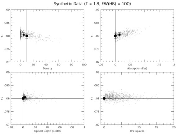
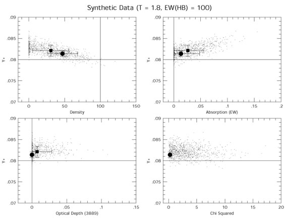
Figure 5 presents the results of modeling of 6 synthetic He I line observations for a single case. The four panels show the results of a density = 10 cm^-3, a_HeI = 0, and (3889) = 0 model. The solid lines show the input values (e.g., He / H = 0.080) for the original calculated spectrum. The solid circles (with error bars) show the results of the ² minimization solution (with calculated errors) for the original synthetic input spectrum. The small points show the results of Monte Carlo realizations of the original input spectrum. The solid squares (with error bars) show the means and dispersions of the output values for the ² minimization solutions of the Monte Carlo realizations.

Figure 5. Results of modeling of 6 synthetic He I line observations. The four panels show the results of a density = 10, aHeI = 0, and (3889) = 0 model. The solid lines show the input values (e.g., He / H = 0.080) for the original calculated spectrum. The solid circles (with error bars) show the results of the 2 minimization solution (with calculated errors) for the original synthetic input spectrum. The small points show the results of Monte Carlo realizations of the original input spectrum. The solid squares (with error bars) show the means and dispersions of the output values for the 2 minimization solutions of the Monte Carlo realizations.

Figure 5 demonstrates several important points. First, our ² minimization solution finds the correct input parameters with errors in He / H of about 1% (less than the 2% errors assumed on the input data, showing the power of using multiple lines). In this low density case, the Monte Carlo results are in relatively good agreement with the input data, with similar sized error bars. There is a small offset to lower densities and a similar small offset to non-zero values of underlying absorption. We found this effect throughout our modeling, that when an input parameter such as underlying He I absorption or (3889) is set to zero, the minimization models of the Monte Carlo realizations (cases with errors) always found slightly non-zero values (although consistent with zero) in minimizing the ². Note that in the lower right panel of Figure 5 that the values of the ² do not correlate with the values of y⁺. The solutions at higher values of absorption and y⁺ are equally valid as those at lower absorption and y⁺.

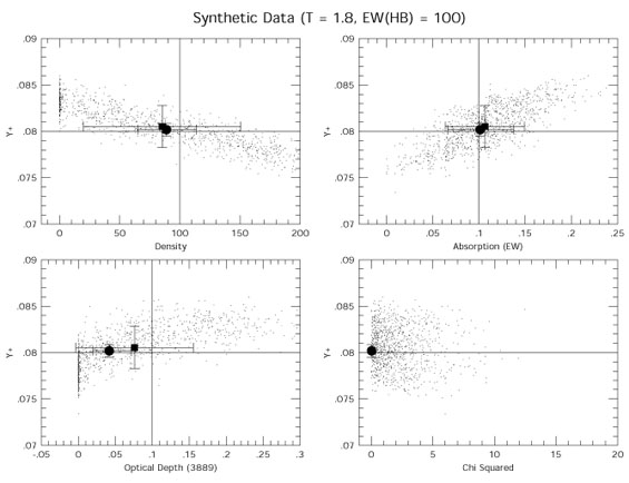
Figure 6 presents the results of modeling of 6 synthetic He I line observations for a case identical to that of Figure 5 with the exception of a higher density of 100 cm^-3. For the n = 100 cm^-3 case, there is a systematic trend for the Monte Carlo realizations to tend toward higher values of He / H. This is because, again, the inclusion of errors has allowed minimizations which find lower values of the density and non-zero values of underlying absorption and optical depth. However, in this case, there is more "distance" from the lower bound of n = 0, and thus more parameter space to allow the effects of the parameter degeneracy to be noticed. Note that the size of the error bars in He / H have expanded by roughly 50% as a result. We can conclude from this that simply adding additional lines or physical parameters in the minimization does not necessarily lead to the correct results. In order to use the minimization routines effectively, one must understand the role of the interdependencies of the individual lines on the different physical parameters. Here we have shown that trade-offs in underlying absorption and optical depth allow for good solutions at densities which are too low and resulting in helium abundance determinations which are too high. This is one of the central results of this study. Again, note that there is no trend in the values of ² with y⁺.

Figure 6. Similar plot to Figure 5 except that the density = 100 as opposed to 10 as in Figure 5.

Table 1 summarizes the results of a number of different test cases like those shown in Figures 5 and 6. Table 1 is grouped into six different cases of input with five different minimization routines. The first two cases correspond those shown in Figures 5 and 6. The other four cases consider non-zero values of underlying absorption, (3889), or both. The first two columns show the results of minimizing on 3 lines (both assuming (3889) is zero and solving for (3889)). The next two columns show the results of minimizing on 5 lines (both assuming zero underlying absorption and solving for the underlying absorption). The last column shows the results of the six line method which was used to produce Figures 5 and 6.

Table 1. Results From Synthetic Spectra

The numbers in the table correspond to the average of the Monte Carlo results and their dispersion. The row labeled He / H gives the results from averaging the He / H abundances from all of the lines (3, 5 or 6), while the "He / H (3)" row gives the He / H values derived from averaging only the three main He I lines (after solving for the physical parameters). Note that the straight minimizations of the input data always returned the input data (except in the cases where an assumption is inconsistent with the input data). Deviations of the Monte Carlo solutions from the input values result because of: (1) inconsistencies between the input data and input assumptions, (2) asymmetries in the Monte Carlo distributions (e.g., in Figure 5, because the absorption is not allowed to go negative, the distribution is truncated on one side, and thus there is a bias to higher values of y⁺), (3) degeneracies between different parameters which result in lower ² values for values of the physical parameters quite far from their input values.

For the first two cases, (no underlying absorption and no optical depth), as expected, the 3 line method constraints on the density are not strong. However the derived helium abundances are consistent, within the errors, with the input values. For the 5 line method, since the first two cases (1 and 2) have no underlying absorption, the method with the correct assumption finds a solution much closer to the correct result (although all solutions are consistent with the correct result, within errors). Again, it is the degeneracy between density and underlying absorption which is responsible for the derived low density and high He abundance. Note, interestingly, that the three line method did not do any worse (in fact it did slightly better) than the 5 line methods, unless we assume a priori the correct answer for underlying absorption (a_HeI = 0). Similarly, assuming = 0 also improves the result in this case for obvious reasons. The six line method, within the errors, gave results consistent with but not equal to the input parameters. Indeed, there is a systematic trend to lower density and some underlying absorption even when there is none. The net result is a higher estimate of the He abundance. This systematic trend can be traced to the degeneracy in the trends imposed by the different input parameters. However, the 6 line method does significantly better than the 5 line method at constraining the underlying absorption (as the 4206 line anchors the values of a_HeI).

We learn more about the various methods when we consider the remaining cases in Table 1. When (3889) 0 (and a_HeI = 0), the five and six line methods give very accurate results although, once again, 4206 is needed to pin down the value of a_HeI and break the degeneracy. When the input value of a_HeI 0, then only the 5 line method which assumes a_HeI = 0 does badly. The 5 and 6 line methods which solve for a_HeI do quite well. Figure 7 shows the results of the Monte Carlo when both and a_HeI 0, and n = 100 cm^-3, i.e., case 6 of Table 1. Thus it is encouraging that in perhaps more realistic cases where the input parameters are non-zero, we are able to derive results very close to their correct values.

Figure 7. Similar plot to Figure 6 except that the underlying absorption is 0.1 Å and (3889) = 0.1.

Indeed, Figure 7 shows many of effects we have been describing in the previous cases. The average of Monte Carlo realizations is remarkably close to the straight minimization for all of the derived parameters (n, a_HeI, and y⁺). However, there is an enormous dispersion in these results due to the degeneracy in the solutions with respect to the physical input parameters. This results in error estimates for parameters which are significantly larger than in the straight minimization. For example, the uncertainties in both the density and optical depth are almost a factor of 3 times larger in the Monte Carlo. When propagated into the uncertainty in the derived value for the He abundance, we find that the uncertainty in the Monte Carlo result (which we argue is a better, not merely more conservative, value) is a factor of 2.5 times the uncertainty obtained from a straight minimization using 6 line He lines. This amounts to an approximately 4% uncertainty in the He abundance, despite the fact that we assumed (in the synthetic data) 2% uncertainties in the input line strengths. This is an unavoidable consequence of the method - the Monte Carlo routine explores the degeneracies of the solutions and reveals the larger errors that should be associated with the solutions.

From the above, we conclude (1) that adding absorption to the minimization routines can lead to much larger regions of valid solution space; (2) the trivial result that assuming no underlying absorption will lead to incorrect solutions in the presence of underlying absorption, (3) that adding an accurate 4026 observation to a minimization solution will provide strong diagnostic power for underlying stellar absorption, and (4) that Monte Carlo models are required to determine the true uncertainties in the minimization results.

5.2. Cases with Systematic Errors in I(3889)

In Section 4, it was shown that 3889 is strongly sensitive to optical depths effects and is required if 7065 is to be a good tracer of density. It was also pointed out that, unfortunately, 3889 is blended with H8 (3890). Thus, in order to derive an accurate F(3889) / F(H) ratio, the F(3890) must be subtracted off and underlying stellar H I (and He I) absorption must be corrected for.

In the methodology of IT98, the contribution to He I 3889 from H I emission is subtracted off by assuming the theoretical value for the H I emission (typically, the He I emission accounts for almost 50% of the blended line). The total emission has to be corrected for underlying stellar absorption, which is assumed to be a constant equivalent width for all of the H I lines. This assumption is a potentially dangerous one. Spectral studies of individual stars show that while this may be a good assumption to first order, the equivalent widths of the higher order Balmer lines are not strictly identical (see, for example, the spectral atlas of Galactic B supergiants of Lennon, Dufton, & Fitzsimmons 1992). Secondly, this correction is usually large (corrected He I 3889 emission line equivalent widths generally lie in the range of 4 to 10Å compared to the underlying absorption which is in the range of 0.5 to 3Å). A good test of the uncertainty in this correction would be a comparison of the corrected higher order (H9 and H10) H I emission line strengths compared to their theoretical values. In Appendix B, we show a few cases in the literature, where these comparisons reveal evidence of a problem.

Here we investigate the possible effects of a systematically low strength of 3889 motivated by the possibility of oversubtracting the underlying H I absorption. We have run identical cases and analyses as in Table 1, but altered the input synthetic spectra by decreasing the relative flux and equivalent width of 3889 by 10%. These results are presented in Table 2. The first two columns are identical (since they are based on only three unaffected lines) and are repeated for comparison. Note that this exercise was motivated, in part, by the systematically low values of He / H derived from 3889 when compared with the main three He I lines in a subsample of the highest quality data from IT98.

Table 2. Results From Synthetic Spectra with He I 3889 10% Low

The 10% drop in 3889 has dramatic effects. From Section 4, and especially Figure 4, it can be seen, that an underestimate of I(3889) will lead to both artificially high values of (3889) and artificially low values of the density. This is born out in inspection of Table 2. Beginning with the cases in which the input values of and a_HeI are 0, we see that the density is grossly underestimated in both input cases with n = 10 and 100 cm^-3. In the low density case, the He / H solutions based on all available lines are low, while the He / H(3) solutions are close to correct. This main effect is due to including the low value of He / H from 3889. However, in the high density case, it is the values of He / H(3) which are in error on the high side. This is due to the underestimate of the density (and thus the corrections for collisional enhancement are too small). Note that the solutions for (3889) have been driven to large values. For both the higher density cases, the density has been underestimated, the (3889) overestimated, and the He / H(3) overestimated.

In Figure 8, we show the results of the 6 line method Monte Carlo for case 2 of Table 2. Here the low density, high (3889), and bias towards higher values of He / H are clear (even higher values would be shown if He / H(3) were plotted). Note that the lower right panel shows that the ² values are all systematically high for this case. It would appear that the ² is a sensitive test to check whether the I(3889) values are systematically biased.

Figure 8. Similar plot to Figure 6 except that I(3889) and EW(3889) are artificially decreased by 10%.

5.3. Cases with Systematic Errors in I(7065)

One of the possible problems of using 7065 is that in a spectrum where the entire wavelength range from 3727 to 7065 is observed in first order, there is the potential for contamination of the red part of the spectrum from blue light in the second order. In principle, if a blue cutoff filter is used (e.g., a CG385 order separation filter) then there should be little contamination blueward of 2 × 3850 Å or 7700 Å. However, order separation filters are not perfect cut-on filters at 3850 Å, but rather start to filter out light above 4000 Å, reach 50% transparency at about 3850 Å and then drop to zero transparency somewhere between 3500 and 3600 Å. Thus, there is potential for some second order contamination for all wavelengths above 7000 Å. If the observed target has a significant redshift, then the He I 7065 is even more susceptible to this problem. The problem is worse for bluer order separation filters (e.g., CG375).

This effect can be quite subtle and there are two separate problems to consider. The first is contamination of the standard star spectrum. If a blue standard star (e.g., a white dwarf) is used for flux calibration, then the far red part of the spectrum detects additional second order blue photons, which, when used to calibrate the spectrograph, results in an overestimate of the red sensitivity of the spectrograph. The second problem occurs in the target spectrum. Here the far red continuum will be contaminated by extra second order blue photons. It is possible that if the blue spectral shape of the standard star is similar to the spectral shape of the target, then these two effects will compensate, giving a rather normal looking red continuum. However, the overestimate of the red sensitivity will result in underestimated emission line fluxes and equivalent widths. Since 7065 lies right at the border of where this effect can become important, it is very important to check for this possibility. This is most easily done by obtaining spectra of both red and blue standard stars and deriving instrument sensitivity curves independently for the two stars. The wavelength at which the two sensitivity curves begin to deviate indicates the onset of second order contamination.

Here we investigate the possible effects of a systematically low strength of 7065. We have run identical cases and analyses as in Table 1, but altered the input synthetic spectra by decreasing the relative flux and equivalent width of 7065 by 5%. These results are presented in Table 3. Note that this exercise was motivated, in part, by the systematically low values of He / H derived from 7065 when compared with the main three He I lines in a subsample of the highest quality data of IT98.

Table 3. Results From Synthetic Spectra with He I 7065 5% Low

In Figure 9, we show the results of the six-line method Monte Carlo for case 2 of Table 3. Case 2 shows the most discrepant results in Table 3, and the six-line method is only better than the five-line method with absorption allowed (but not constrained by 4026. Here it can be seen clearly that the solutions all favor lower density, and thus higher He / H. The trade-off between low density and high values of underlying absorption is clearly shown. Interestingly, the values for ² are relatively low and quite satisfactory. Clearly the ² is not a good diagnostic of an underestimated I(7065), as the degeneracies allow mathematically acceptable solutions.

Figure 9. Similar plot to Figure 6 except that I(7065) and EW(7065) are artificially decreased by 5%.

In Figure 10, we show the results of the six-line method Monte Carlo for case 6 of Table 3. In this case of a small amount of optical depth and a small amount of underlying absorption, the solutions do a pretty good job of finding the correct range of density, optical depth, and underlying absorption. The underestimated 7065 has resulted in a bias toward lower density, which has resulted in a bias toward larger He / H, but the effect is not very large. The main effect is the size of the error bars. Here it is clear that Monte Carlo errors in He / H are about 3 times larger than the errors from a straight minimization. Note again that the ² values are generally small.

Figure 10. Similar plot to Figure 7 except that I(7065) and EW(7065) are artificially decreased by 5%.