2. THEORETICAL BACKGROUND

For the majority of this review, we will work in the context of the Big Bang model. In order to set a common language and notation, we briefly review the relevant points of Big Bang cosmology to which we will find ourselves referring. The Big Bang model itself is discussed in Section 2.1, in which we define the basic parameters of an homogeneous and isotropic expanding universe, and write down the equations for their evolution. Section 2.2 gives the evolution equations for perturbations in such a homogeneous universe, and Section 2.3 discusses the power spectrum of these perturbations, and introduces the concept of dark matter. Section 2.4 discusses models for the relative distribution of galaxies and dark matter in the context of the biasing paradigm. Section 2.5 summarizes the outstanding questions we would like to address with the observations.

2.1. The Big Bang Model and its Parameters

It is an observational fact that all galaxies (with the exception of galaxies in the Local Group and a few galaxies associated with the Virgo Cluster) have positive redshifts, and it is observed that redshifts are proportional to distance (Section 3.6). This is interpreted as due to the expansion of the Universe. The Cosmological Principle, as formulated originally by Einstein, states that on large enough scales (to be quantified below) the Universe is homogeneous and isotropic; this model together with the tenets of general relativity leads to the prediction that we do not live in a static Universe ⁽¹⁾ In particular, the Cosmological Principle implies that the covariant line element between two points is given by:

(3)

where a(t) is the scale factor. Our observation that the universe is expanding means that a(t) is an increasing function of time. The comoving distance l between any two points taking part in the Hubble expansion is a constant; the proper distance between two points is the quantity s at a given constant time t, i.e., such that t = 0. Comparing with Eq. (1), we see immediately that

(4)

where the subscript 0 refers to values of quantities at the present time t₀. Indeed, the quantity /a is not constant with time, and thus neither is the Hubble Constant; however, at any given time, it is independent of position and direction.

Consider two observers separated by a proper distance l small compared with the distance to the horizon. By Hubble's law, they are moving apart from one another at a speed given by v = / a l. Now consider a plane wave of radiation, with definite wavelength as measured by the first of the observers, traveling towards the second. The second observer will observe this radiation to be shifted by the first-order Doppler shift (because v << c) to a wavelength

(5)

Thus, recognizing that the proper time required for the radiation to travel the distance l is t = l /c, and taking l -> 0, we find

(6)

or

(7)

The redshift of a galaxy z is defined as

(8)

where ₀ is the wavelength of a plane wave emitted by the galaxy at the time of emission (the rest wavelength), and (t) is the wavelength of the plane wave at the present (the observed wavelength). Thus the redshift and the scale factor are directly linked:

(9)

At low redshifts, the recession velocity of a galaxy is simply given by cz. At high redshifts, this expression clearly breaks down, and one must go to general relativistic generalizations of it.

Under the assumption that the universe is homogeneous and isotropic, the line element can be expressed in spherical coordinates:

(10)

This is called the Friedman-Robertson-Walker metric, after the men who first wrote it down. The quantity k is the curvature constant, an integration constant of Einstein's equations ⁽²⁾ Thus k = 0 corresponds to a Euclidean geometry for the three spatial dimensions; this is called a flat universe.

Dynamical equations for the scale factor a follow from the metric, together with the equations of general relativity and the ideal fluid approximation ⁽³⁾ One finds (e.g., Chapter 15 of Weinberg 1972 ) two equations:

(11)

and

(12)

In these equations, G is Newton's gravitational constant, is the (non-relativistic) mass density of the universe, p is the pressure, H is the Hubble Constant (compare with Eq. 4), where the lack of a subscripted 0 indicates that it is a function of time, and is the Cosmological Constant.

In the present universe, non-relativistic matter completely dominates the energy density of the universe, making the pressure term negligible; we drop it from now on. In this zero-pressure limit, mass conservation implies a^-3(t). The wavelength of any relativistic species will be redshifted with the expansion of the universe; to the extent that the number of particles of this species is preserved, the energy density in relativistic species drops as a^-4(t). The Cosmic Microwave Background (CMB), isotropic radiation with a pure black-body spectrum and a temperature of T₀ = 2.735°K, represents such a relativistic species. The energy density in the CMB today is negligible relative to the density in non-relativistic matter, but because of its faster fall-off with a, it dominated the energy density of the universe for z > 2.4 × 10⁴ ₀ h². The CMB will not be reviewed thoroughly here, although we will find ourselves referring to it often. See Efstathiou (1991) , Peebles (1993) , and Partridge (1994) for recent reviews.

Setting the Cosmological Constant to zero for the moment, and dropping the pressure term, Eq. (12) can be written:

(13)

For k negative or zero, the right hand side, and therefore ²(t), stays positive-definite. We know that (t) is positive now (the universe is observed to be expanding, not contracting) and thus a(t) will continue to increase for all time. This is what we call the open or flat universe. However, if k is positive, there will be some time in the future at which the second term on the right hand side of Eq. (13) balances the first term, and thus ²(t) returns to zero. As is negative-definite (Eq. 11) this means that (t) changes sign, and a(t) begins to decrease, eventually reaching zero. This is a closed universe. The controlling factor deciding the fate of the universe is the density; the division between the open and closed universe happens at the critical density, whose current value is:

(14)

Thus we define the Cosmological Density Parameter ₀ as

(15)

whose value is less than unity for an open universe, greater than unity for a closed universe, and exactly unity for a flat universe. If we re-introduce the Cosmological constant, we get a flat universe (k = 0) in the case that ₀ + = 1, where

(16)

is the contribution to the cosmological density due to vacuum energy. Of course, in this case, the concepts of open and closed universes become more complicated, because can change sign. See Harrison (1981) for a complete inventory of cosmological models.

We can use this line of reasoning to peer into the past as well. As is negative-definite (for = 0, as we will assume) and is positive-definite, then at some finite time t in the past a(t) = 0. This is the origin of the concept of the Big Bang: the dynamical equations for a(t) indicate that the universe was of infinitesimal extent some finite time in the past. Let us define that time t = 0. We can now ask for the age of the universe (Weinberg 1972 ):

(17)

As we could have guessed from the units, the present age of the universe is proportional to H₀^-1, with a numerical coefficient which is a decreasing function of ₀ . The corresponding equations for 0 universes are non-analytic, and will not be presented here.

We need one further definition, the acceleration parameter ⁽⁴⁾ , defined at the present time:

(18)

where the second equality follows directly from Equations 11 and 12. The acceleration parameter is a measure of relativistic effects in the relation between observables; thus, for example, the first-order corrections to Eq. (1) are proportional to q₀.

This completes our survey of the global structure of space-time in a homogeneous and isotropic universe. The cosmology is defined by the following numbers:

- ₀ , the cosmological density parameter;

- H₀, the Hubble constant;

- , the cosmological constant;

- q₀, the acceleration parameter, and

- t₀, the present age of the universe.

These parameters are not independent of one another in the context of the Big Bang model, as we have seen, but each are measured or constrained by a variety of different observations. It is one of the important tests of Big Bang cosmology that one find consistency between the values found for the different parameters. We will put the greatest emphasis in this review on measurements of ₀ , because this is the quantity that can best be constrained with analyses of redshift and peculiar velocity surveys.

Standard Big Bang cosmology has built into it a number of apparent paradoxes. The first is often referred to as the horizon problem: the size of causally connected regions at the time of recombination subtends only a few degrees on the sky, leaving the large-scale isotropy observed in the CMB unexplained: this must be taken as an (arbitrary) initial condition. The second is the so-called flatness problem: ₀ = 1 is an unstable solution to the evolution equations, in the sense that the fact that we observe ₀ to be within an order of magnitude of unity today requires that it be very finely tuned in the early universe.

There is a class of cosmological models under the general rubric of the inflationary paradigm, which addresses these problems, and predicts tight constraints on the parameters of the Big Bang model. Inflation is reviewed thoroughly in Chapter 8 of Kolb & Turner (1990) . In its simplest form, the inflationary model posits a period in the very early universe when a super-cooled phase transition caused the vacuum energy density to become dominant; Eq. (12) then implies that the scale factor grows exponentially. If this exponential expansion continues long enough for the curvature term to become exponentially small, the flatness problem is solved; the result is a universe that is globally flat (i.e., k = 0 or ₀ + = 1). Moreover, as the observable universe inflated from a region that was causally connected and in thermal contact, the homogeneity and isotropy of the universe (the horizon problem) are explained. The inflationary model also predicts a scale-invariant spectrum of adiabatic density fluctuations ⁽⁵⁾ , a subject to which we turn in Section 2.3 after a discussion of gravitational instability theory.

The inflationary prediction of a flat universe is apparently in direct contradiction with measurements of the total mass density of the universe, at least until recently. Measurements of the luminosity density of the universe (cf., Section 3.4) imply that the mass density of the universe in stars is only ~ 0.01 (Section 3.5). There is abundant evidence for non-luminous matter associated with galaxies and clusters of galaxies, whose total contribution is as much as ₀ ~ 0.2 (cf., Faber & Gallagher 1979 ; Kormendy & Knapp 1987 ; Trimble 1987 ). The inflationary prediction of ₀ = 1 in a universe without a cosmological constant requires that there be additional dark matter distributed on scales larger than that of clusters; indeed, as we shall see in detail later in this review, there is recent evidence from large-scale flows that ₀ is larger than that inferred from dynamics within clusters. The material which makes up the dark matter, however, remains completely unknown. The physical properties of the dark matter greatly influences the distribution of matter on large scales, and thus redshift surveys of galaxies have the potential to constrain the form of dark matter. In order to explore these issues, we need a theory for the growth of structure in the presence of gravity.

2.2. The Gravitational Instability Paradigm

The Big Bang model as outlined in the previous section explicitly assumes a homogeneous and isotropic universe. We believe that the Cosmological Principle does in fact hold on the largest scales (for reasons that will be discussed in Section 5.5), and that at early times the universe was very close to homogeneous. However, we observe structure all around us: from planets, to galaxies, to superclusters of galaxies, matter tends to aggregate and form structures, rather than distribute itself uniformly. One of the great questions facing cosmology is how this structure came to be. The widely accepted view is that small density fluctuations present in the beginning grew by gravitational instability into the structures that we see today. In this section, we briefly review the theory of gravitational instability in an expanding universe.

One starts by writing down the equations of mass continuity, force, and gravitation in an expanding universe, in proper coordinates (ignoring relativistic effects):

	(19)
	(20)
	(21)

Here is the mass density field, v is the velocity field, is the gravitational potential, and we have dropped terms depending on pressure, which we assume are negligible. All spatial derivatives are with respect to proper distance. If we expand these equations to first order in all quantities measuring departure from uniformity, convert to comoving coordinates, and subtract the zeroth order solutions ⁽⁶⁾ , the first two equations simplify to

	(22)
	(23)

where is the dimensionless density contrast,

(24)

and ₀ is the mean mass density. Taking the time derivative of the continuity equation and substituting into the divergence of the force equation yields, with the Poisson equation (Eq. 21):

(25)

Because Eq. (25) is a second-order partial differential equation in time alone, we can separate the spatial and temporal dependences, and write:

(26)

where D₁ and D₂ are growing and decaying modes, respectively. We will be using the growing mode throughout this review; it is given by

(27)

In the general case of a non-vanishing cosmological constant, this integral is not analytic. For = 0 models, however, analytic expressions for D₁(t) and D₂(t) can be obtained (Section 11 of Peebles 1980 ). A particularly simple solution exists in the special case of a flat universe, in which a(t) t^2/3 (Eq.17), and the right hand side of Eq. (25) is simply 3/2 ( / a)², so we find:

(28)

which has an analytic solution in power laws ⁽⁷⁾ of t:

(29)

More generally, the solutions depend on ₀ ; in particular, the growth is faster for increasing ₀ . For ₀ < 1, the expansion of the universe (the drag term represented by 2 / a ð / ðt in Eq. 25) dominates the gravitational attraction of the matter, and the clustering freezes out (i.e., it stops growing) at z 1 / ₀ - 1. A full discussion of these solutions, including the effects of pressure which is important in the early universe, will take us too far afield; cf. Chapter 9 of Kolb & Turner (1990) for more details.

If we wait until late times, the growing mode of Eq. (26) will dominate, and we can rewrite Eq. (22) as:

(30)

where

(31)

We are still in comoving coordinates, as indicated by the a on the right hand side of Eq. (30). The expression for D₁, and therefore for f, is a function of ₀ and . A good approximation in the general case is given by Lahav et al. (1991) :

(32)

other approximations can be found in Peebles (1984) , Regös & Geller (1989) , Lightman & Schechter (1990) , Martel (1991) , and Carroll, Press, & Turner (1992) . Thus the influence of on dynamics at low redshift is minimal (Lahav et al. 1991 ). Eq. (30) can be inverted via the methods of electrostatics in the usual way to yield, after returning to proper coordinates ⁽⁸⁾ :

(33)

Eq. (33) reveals the physical content of this first-order expansion: linear perturbation theory states that peculiar velocities are proportional to gravitational acceleration. We will find ourselves using Eqs. (30) and (33) throughout this paper. These equations can be generalized using higher-order perturbation theory; we will introduce these results when needed.

If we measure the quantity r in units of km s^-1, then H₀ 1, and we see that a comparison of the velocity field v(r) and density field (r) gives a direct measure of f ( ₀ , ). One of the central themes of this review will be exploiting this comparison to put constraints on f.

Linear theory makes the assumption that the change in comoving position of galaxies as the universe expands is negligible. Zel'dovich (1970) made an important extension of linear theory by assuming that the difference between the Lagrangian position q and Eulerian position x of a particle in a gravitating system is separable in space and time:

(34)

where D₁(t) is the growing mode in linear theory (Eq. 27) and , which determines the amplitude of the velocity field, is proportional to the gradient of the gravitational potential. See Shandarin & Zel'dovich (1989) for a review of the full ramifications of this deceptively simple equation. This approximation is used as a basis for several of the non-linear schemes described in Section 5.2.2.

2.3. Power Spectra, Initial Conditions, and Dark Matter

We have seen that initially small perturbations grow by gravitational instability. It remains to characterize the distribution with scale of those initial perturbations. Let us define the Fourier Transform (k) of the fractional density field (r) at some early time t such that:

(35)

(Care needs to be taken when comparing the results of different authors, as there is inconsistency in the literature about where the factors of 2 go in the definition of the Fourier Transform.) Because of the isotropy assumed in the Cosmological Principle, the statistical properties of (k) are independent of the direction of , and so it makes sense to define a power spectrum P(k):

(36)

where ^D is a Dirac delta function, and the averaging on the left-hand side is over directions of k. As Bertschinger (1992) makes clear, P(k) is a power spectral density, and thus represents the power per unit volume in k-space. One often sees the power spectrum defined as P(k) <|(k)|²>, but this is incorrect (at least for the Fourier Transform convention we've adopted), as can be seen by comparing the units of the two expressions: the power spectrum has units of volume, as does .

The quantity (k) is complex, and thus P(k) is a complete statistical description of the density field ⁽⁹⁾ only if the phases of (k) are random. This is a natural prediction of inflationary models, and is often called the random-phase hypothesis. By the Central Limit Theorem and Eq. (35), random phases imply that the one-point distribution function of (r) is Gaussian ⁽¹⁰⁾ , so the random-phase hypothesis is often also referred to as the Gaussian hypothesis. Random phases can strictly hold only in the limit of very small perturbations: (r) cannot be smaller than -1 (Eq. 24), but has no upper bound, and therefore it develops a positive skewness (about which we will have much more to say in Section 5.4) as perturbations grow by gravitational instability. Until the lower bound on becomes important, linear theory holds, and because gravitational growth of perturbations is independent of scale in linear theory, the shape of the power spectrum is independent of time.

One way to quantify the density fluctuation field is in terms of the mass fluctuations within a spherical window of radius R:

(37)

where W(R) is the window function used; (kR) is its Fourier Transform. For a tophat window function, which is unity out to some radius R, and then drops to zero,

(38)

where j₁(x) (sinx - xcosx) / x² is the first spherical Bessel function. This is very crudely a step function to k 1 / R. This implies that characteristic mass fluctuations on a scale k = 1 / R are given roughly by

(39)

It is interesting to compare the mass fluctuations within a sphere of radius R with the corresponding fluctuations in the bulk flow velocity within the same sphere. Using Eq. (30) and following a derivation very similar to that in Eq. (37), one finds:

(40)

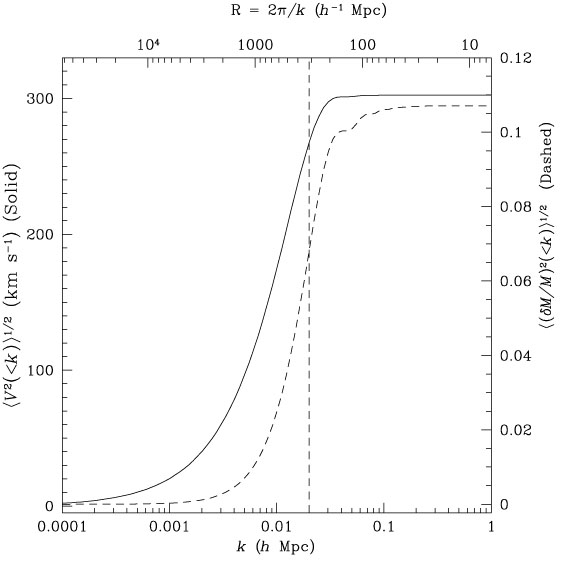
which differs from Eq. (37) with two fewer powers of k in the integrand. This means that the peculiar velocity field on a given scale is sensitive to components of the power spectrum on larger scales than is the density field, and thus is a useful probe of the largest-scale power. We illustrate this in Fig. 1, which compares the cumulative contribution to the integrals in Eqs. (39) and (40) for wavenumbers smaller than k. This calculation used a top-hat window of radius 50 h^-1 Mpc, and assumed a standard Cold Dark Matter model (see below). The rms velocity includes contributions from much larger scales than do the rms mass fluctuations.

Figure 1. The solid curve shows the square root of the contribution to the mean squared bulk flow within a tophat of radius 50 h-1 Mpc as a function of the lower cutoff in k, for a standard CDM model. The dashed line is the square root of the contribution to the mean squared mass fluctuations (right-hand scale). Note that the velocity field includes much more contribution from small k (large scales).

The simplest inflationary models predict a so-called scale-invariant power spectrum, given by

(41)

so-called because the potential fluctuations on a scale at the time that is equal to the horizon size, are independent of for this spectrum (cf., Kolb & Turner 1990 ). This form was in fact predicted well before inflation had been suggested (Peebles & Yu 1970 , Harrison 1970 , Zel'dovich 1972 ), as it is unique among power-law power spectra in avoiding divergences at large and small k in various observable quantities.

The pure power-law power spectrum thought to exist in the early universe is sometimes called the primordial power spectrum. However, the power spectrum that is directly observable is that which holds following the epoch at which the energy densities in relativistic and non-relativistic particles are equal. The equations of gravitational instability we worked out above hold only for pressureless (i.e., non-relativistic) matter; in the relativistic case, the pressure of the matter is such as to retard the growth of perturbations on all scales within the radius of the universe. Thus perturbations on scales smaller than the horizon (the scale over which the universe is causally connected, ~ ct) can only grow after non-relativistic matter becomes dominant, and this is thus a convenient time at which to characterize the power spectrum.

While perturbations cannot grow on scales smaller than the horizon during the radiation-dominated era, they can and do grow on scales larger than the horizon. After the epoch of matter-radiation equality, perturbations on sub-horizon scales start to grow, although at a different rate ⁽¹¹⁾ The combination of these two effects causes a bending in an originally pure power-law power spectrum on the scale of the horizon size at matter-radiation equality. The index of the power law decreases by four over this bend. Thus following matter-radiation equality, the power spectrum which is proportional to k¹ on large scales bends over to become k^-3 on small scales. One quantifies this in terms of a transfer function, whose square is the quantity by which the primordial power spectrum is multiplied to generate the final power spectrum.

The power spectrum we have described is generic for universes in which the dark matter is non-relativistic (or "cold") when a galaxy mass is contained within the horizon; its form depends principally on the horizon size at the epoch of matter-radiation equality, which scales as 1 / ₀ h². The so-called Standard Cold Dark Matter model (CDM) goes further and invokes inflation to give ₀ = 1 and Eq. (41) for the primordial power spectrum; the Hubble Constant is set to H₀ = 50 km s^-1 Mpc^-1 in order to get an age of the universe in concordance with the ages of the oldest globular clusters (Section 9.6). Although the CDM model has been very popular ever since it was first proposed (some of the early important papers include Peebles 1982 , Blumenthal et al. 1984 , and Davis et al. 1985 ), due to its naturalness, lack of free parameters, and successes in predicting many of the observed properties of galaxies, there exists no compelling model invoking particles or physical processes known to exist that predicts any form of CDM. Particle physicists have come up with a number of hypothetical particles which could constitute the CDM, axions and the lightest supersymmetric partner to the photon among the most popular at the moment (cf. Primack, Seckel, & Sadoulet 1988 ; Kolb & Turner 1990 ).

The power spectrum of the Cold Dark Matter model has been calculated numerically by a number of workers (Peebles 1982 , 1984; Bond & Efstathiou 1984 ; Efstathiou, Bond, & White 1992 ), and fit to various functional forms; Efstathiou et al. (1992) give:

(42)

where A is a normalizing constant, k is measured in units of h Mpc^-1, ₀ h, and n is the power-law index of the primordial power spectrum. The quantity h is the Hubble constant in units of 100 km s^-1 Mpc^-1. Thus Standard CDM sets = 0.5; models with smaller have more power on large scales. The quantity is inversely proportional to the Hubble radius at matter-radiation equality, and thus sets the scale at which the power spectrum bends over. This equation (and the equality between and ₀ h) holds only in a universe with a negligible contribution of baryons to ₀ . The normalization for the case of n = 1 and ₀ = 1 (standard CDM) can be written (Bunn, Scott, & White 1995 ; White, Scott, & Silk 1994 ):

(43)

where ₀ is the conformal time at the present, <Q> is the measured quadrupole anisotropy of the CMB background, and T₀ is its measured temperature.

There is another physical effect that can come in. We have assumed that the dark matter is cold at the epoch when a galaxy mass is contained within the horizon. However, imagine that the dark matter is made up of neutrinos with a mass around 100 eV (already ruled out for _e, but well within experimental bounds for _µ and ). It can be shown from considerations of thermodynamic equilibrium in the early universe that the number density of neutrinos in this case would be enough to close the universe (i.e., = 1). Moreover, neutrino dark matter would be relativistic at a time when a galaxy mass was enclosed within the horizon, and thus in their free-streaming, would wash out any perturbations on scales comparable to the horizon scale at that epoch. The consequence is a power spectrum that cuts off exponentially on small scales. The evolution of large-scale structure in such a Hot Dark Matter model, or HDM, is very different from that in CDM. Because there is no power on the scale of galaxies in the HDM model, larger scale structures collapse first in pancakes, that then fragment later to form galaxies. This is often referred to as the top-down scenario. In CDM, on the other hand, there is power on galaxy scales, and galaxies form first, thereafter clustering into larger scales. Indeed, collapse is simultaneous for all scales for which P(k) k^-3 (Eq. 39). This is referred to as hierarchical clustering, or the bottom-up scenario.

The mass perturbations predicted by inflation arise from perturbations in the gravitational potential, and thus relativistic and non-relativistic components fluctuate in tandem. These are called adiabatic fluctuations, in contrast with isocurvature fluctuations, in which the two fluctuate in opposite senses to give no net fluctuations in the mass density. The Primordial Baryon Isocurvature models (PBI), first suggested by Peebles (1987; cf. Bardeen, Bond, & Efstathiou 1987 ), invoke neither a hypothetical new particle (as in CDM) nor a hypothetical mass for a particle now believed to be massless (as the neutrino in HDM). Rather, baryons dominate the mass density of the universe. The PBI models characteristically show a strong peak in the power spectrum at the Jeans length at the epoch of matter-radiation equality.

The power spectra of a variety of models are shown in Fig. 2, based on a similar figure in Strauss et al. (1995) . Shown are Standard CDM, HDM, and two variants of the PBI model; note the bump on large scales in the PBI models. Also shown are two variants of Standard CDM, one with = 0.3 (LCDM, this increases the epoch of matter-radiation equality, and therefore the wavelength of the turnover in the power spectrum), and one which invokes somewhat non-standard inflationary models to assume a primordial power spectrum given by P(k) k^0.7 (Tilted CDM, or TCDM). Finally, we show a hybrid model with a roughly 2 : 1 mixture of CDM and HDM (C+HDM). The parameters for these models are given in Table 1. We will discuss these models in detail in Section 9.1.

Figure 2. The power spectra in seven models of large-scale structure: Standard CDM, Tilted CDM (Tilted CDM), = 0.3 CDM (LCDM), HDM, Mixed Dark Matter (C+HDM), and two variants of the PBI model. All are normalized to the COBE observations.

Table 1. The Parameters of the Power Spectra

Model	0 a	8 b	H0 c	n d or m e	x f
Standard CDM	1.0	1.05	50	1.0	0.0
HDM	1.0	0.86	50	1.0	0.0
PBI 1	0.2	0.90	80	-0.5	0.1
PBI 2	0.3	1.02	50	-1.0	0.1
LCDM	0.3	0.67	67	1.0	0.0
TCDM	1.0	0.50	50	0.7	0.0
C+HDM	1.0 g	0.67	50	1.0	0.0
a All models are spatially flat so that 0 = 1 - 0.
b rms fraction density fluctuations within 8 h-1 Mpc spheres.
c Hubble Constant in units of km s-1 Mpc-1.
d Adiabatic primordial spectral index.
e Isocurvature primordial spectral index.
f Ionization fraction.
g CDM = 0.7, HDM = 0.3.

All of these models are normalized to the anisotropies in the CMB on a scale of 10°, as measured by the Cosmic Background Explorer (COBE) (Smoot et al. 1992 , Wright et al. 1992, Efstathiou, Bond, & White 1992), based on the assumption that the observed anisotropies are due to potential fluctuations at the surface of last scattering (the Sachs-Wolfe (1967) effect). Note that inflationary models (or for that matter, other competing models for the generation of fluctuations in the early universe) are not specific enough to predict the amplitude of the fluctuations; we simply do not know the relevant particle physics well enough. Thus COBE provides the only unambiguous way to normalize power spectra ⁽¹²⁾ Indeed, in the pre-COBE days, the normalization of power spectra was a free parameter which was only weakly constrained by galaxy clustering (Eq. 52). A thorough discussion can be found in Efstathiou (1991) and Peebles (1993) .

2.3.1. The Correlation Function

The autocorrelation function, or, more commonly, the correlation function of the mass density field, is one of the most powerful methods of quantifying galaxy clustering. It is defined by

(44)

where the average is over position x and isotropy guarantees that (r) is independent of the direction of r. Eq. (44) is only applicable for continuous density fields; for a point process such as the distribution of galaxies, we define (r) operationally as the mean excess number of galaxy pairs at separation r, over that expected for a pure Poisson distribution. That is, the mean number of galaxies in a spherical shell a distance r from a given galaxy of thickness r is given by

(45)

where n is the mean number density of galaxies. If we expand the 's in Eq. (44) in inverse Fourier Transforms, we find:

(46)

Thus the correlation function and the power spectrum form a Fourier Transform pair. We discuss the application of (r) in much greater detail in Section 5.1. Just as for the power spectrum, the correlation function gives a complete statistical description of the density field for a Gaussian field; all higher-order correlations are zero. Thus higher-order correlations are a measure of non-Gaussianity, as we discuss in Section 5.4.

2.4. The Relation Between the Mass and Galaxy Density Fields

Our discussion thus far has been quite abstract; galaxies have been mentioned only in passing. However, it is galaxies that we observe directly, while we believe that most of the material of the universe is made up of dark matter; we need to make a connection between the galaxies and the mass density field. The simplest assumption, and one that was implicitly made until the last decade, is that the distribution of galaxies is a mirror of the distribution of dark matter. This could come about, for example, if each galaxy were surrounded by a halo of dark matter with total mass in proportion to the (visible) luminosity of a galaxy, with no extra component of dark matter either smoothly distributed, or lying in clumps with no associated visible matter. However, there is very little evidence that this is true, and some indirect evidence that it is false. For example, one could imagine that a component of the dark matter is distributed like that of the galaxy field smoothed on scales of 5 h^-1 Mpc, and does not follow the details of the galaxy distribution on smaller scales. If this were the case, one would get a misleading impression of the small-scale distribution of dark matter from studying galaxies. A specific model for this sort of effect was first suggested by Kaiser (1984) , in which galaxies form only at the high-density peaks of the mass density field. The galaxy distribution is then said to be biased with respect to the mass distribution. The term biasing is used to refer to a number of different but related effects.

The original argument of Kaiser (1984) was concerned not with the biasing of galaxies relative to dark matter, but of clusters of galaxies relative to galaxies: clusters of galaxies are likely to be produced where the initial density contrast, smoothed on larger scales, is high, and therefore is likely to produce a higher than average density of other clusters. The result is a stronger correlation function (Eq. 44) of clusters than that of galaxies, as is indeed observed (Bahcall & Soneira 1983 ; Bahcall & West 1992 ). Thus this form of bias is known to exist.

It was then realized that a similar effect could cause galaxies to be biased relative to the underlying dark matter (Bardeen et al. 1986 , Davis et al. 1985 , Peacock & Heavens 1985 ), causing the clustering of the former to be stronger than that of the latter, and decreasing the apparent value of ₀ from dynamical studies. The so-called peaks biasing model originally proposed by Kaiser (1984) makes a definite prediction for the relation between the correlation function of the galaxies and dark matter, at least on large scales:

(47)

where b is the biasing parameter, which is (approximately) a constant, independent of scale, related to the threshold above which galaxies are presumed to have formed. In practice, we will often assume the much more specific linear biasing model, in which

(48)

This is in fact the intuitive definition of biasing that most people have, in which a constant of proportionality relates the dark matter density field to that of the galaxies. Note that in practice, the galaxy distribution is a point process, not a continuous field, and thus the bias defined as above must always make reference to a smoothing length. Eq. (48) implies Eq. (47) through Eq. (44), although the converse is certainly not true. Furthermore, for b > 1 (as is usually assumed) Eq. (48) cannot be strictly true, because both _galaxies and _{dark matter} are limited below by -1, and thus one occasionally sees models like:

(49)

which gets around this problem. Weinberg (1994; cf., Coles 1993 ) has shown empirically that in a wide range of models which invoke local biasing, i.e., in which

(50)

the ratio of the fluctuations (R) in the galaxies and dark matter is independent of scale R on scales larger than 5 h^-1 Mpc. This of course will not hold in non-local biasing models, in which galaxy formation is influenced by events many Mpc away (Babul & White 1991 ; Bower et al. 1993); in these schemes, the ratio of the amplitude of dark matter and galaxy fluctuations can be a strong function of scale.

Any given prescription relating _galaxies to _{dark matter} is expected to hold only in the mean; at any given point in space, there will be fluctuations around this mean in the relation between the two. A complete model of biasing must specify the distribution of these fluctuations.

To the extent that the linear biasing model holds, comparisons of peculiar velocities and gravity via Eq. (30) will not be able to constrain the quantity f, but rather the combination

(51)

Thus our ignorance about the relative distribution of galaxies and dark matter translates directly into ignorance of the value of ₀ . Note in particular that for b > 1, as is usually assumed, ₀ = 1 models can be reconciled with observed low values of . Thus biasing is often invoked to explain why some dynamical observations imply a value of ₀ substantially below the inflationary prediction of unity (Section 8.1).

An early review of the biasing model and specific physical models which predict biasing can be found in Dekel & Rees (1987) ; recent work has found biasing of the galaxies relative to the dark matter in numerical simulations of galaxy formation and the growth of structure in an expanding universe (e.g., White et al. 1987 ; Gelb & Bertschinger 1994a ; Cen & Ostriker 1992b ; Katz, Hernquist, & Weinberg 1992 ).

If galaxies can be biased with respect to the underlying dark matter, different populations of galaxies can in principle be biased with respect to one another. We know that this holds on small scales for elliptical and spiral galaxies: although elliptical galaxies make up roughly 15% of the population of galaxies in the field, they are by far the dominant population in the cores of rich clusters (Hubble 1936 , Oemler 1974 , Dressler 1980a, b, Dressler 1984 , Postman & Geller 1984 , Whitmore, Gilmore, & Jones 1993). This is reflected in a steeper correlation function of ellipticals relative to spirals (Davis & Geller 1976 , Giovanelli, Haynes, & Chincarini 1986 ). We refer to this as a form of relative biasing of two galaxy populations, and will discuss further observational evidence for this below.

Finally, the term biasing is occasionally (mis)-used to refer to the normalization of the power spectrum. It is observed that the variance of optically selected galaxy number counts is approximately unity within spheres of radius 8 h^-1 Mpc (Eq. 37, Davis & Peebles 1983b ) and thus the bias can be defined as

(52)

at R = 8 h^-1 Mpc, with W given by Eq. (38). This definition is consistent with that in Eq. (48) only to the extent that the variance in galaxy counts at R = 8 h^-1 Mpc is actually unity, whereas in fact it varies from sample to sample. Thus we will shun this definition of b in this paper.

2.5. Outstanding Questions

This finishes our overview of the theoretical framework within which we will interpret the results of redshift and peculiar velocity surveys. As a form of summary, we list the issues we would like to address with observational data:

1. The Friedman-Robertson-Walker metric is characterized by a number of parameters: ₀ , H₀,, q₀, and t₀, which, although not independent in the model, are constrained observationally by quite different methods. Redshift and peculiar velocity surveys have the most power to constrain ₀ (mostly through Eq. 30), and that is what we will concentrate on for this review.
2. The gravitational instability model is compelling, but needs to be tested observationally. Linear theory and gravitational instability imply a unique relation between the mass and velocity fields (Eq. 30), furnishing one such test.
3. The power spectrum following the epoch of radiation-matter equality is of paramount importance for determining the evolution of large-scale structure in our universe. Moreover, as we have seen, it can give vital clues as to the form and amount of the dark matter. We will attempt to constrain it with observations.
4. The power spectrum discussed above is a complete statistical description of the mass fluctuations in the early universe only to the extent that the Fourier modes had random phases. We will see that there do exist direct observational tests of this from the nearby galaxy distribution.
5. The physical processes by which galaxies formed are very poorly understood. Redshift and peculiar velocity surveys can put constraints on the relative distribution of galaxies and dark matter; this relative distribution ultimately must be predicted by galaxy formation models.
6. At the end, we wish to step back and ask whether the various observational constraints we have found allow a coherent picture consistent with the theoretical framework. That is, are our observations consistent with the Big Bang model, with structure forming via gravitational instability? To what extent can we rule out competing models?

At this point, we are ready to start addressing these questions with observations of the galaxy distribution and velocity field at low redshifts.

¹ The introduction of a cosmological constant does allow solutions indicating a static Universe, but these solutions are unstable. Back.

² The curvature constant is sometimes written in the form ± 1 / R² because in a closed universe, a₀R can be interpreted as the radius of the universe (cf. Eq. 5.9 of Peebles 1993 ). Back.

³ These equations may also be derived heuristically following a purely Newtonian argument (cf. Chapter 5 of Peebles 1993 ). Back.

⁴ Some authors refer to q₀ as the deacceleration parameter. Back.

⁵ There do exist variants on the standard inflationary model which predict other forms for the density fluctuation spectrum, and which predict noticeable curvature; see the references at the end of Section 8.5 of Kolb & Turner (1990) . Back.

⁶ The subtraction of the zeroth order solution involves some subtleties having to do with the gravitational potential of a uniform universe; these are discussed further in Section 8 of Shu (1992) . Back.

⁷ Pressureless gravitational growth in a non-expanding universe is quite different: the drag term is not present, and perturbations grow exponentially. Back.

⁸ One has the freedom to add an arbitrary divergence-free term to the right-hand side of Eq. (33). This term corresponds to the decaying solution, and thus will be negligible at the present. Back.

⁹ That is, the multi-variate distribution function of (k_i), i = 1,..., N is a multi-variate Gaussian with covariance matrix given by Eq. (36). Back.

¹⁰ There are classes of models whose initial conditions are explicitly non-Gaussian: among them are models with initial seeds of gravitational growth (primordial black holes, cosmic string loops and wakes, monopoles, textures), and with initial explosions. We will have little to say about these models in this review. Back.

¹¹ This is true for the dark matter, which does not couple with the radiation. However, baryonic matter is still ionized at the epoch of matter-radiation equality, and thus is tightly coupled to the photons. Therefore, fluctuations in the baryonic component cannot grow until recombination. These considerations are of great importance in quantifying fluctuations in the CMB on small scales. Back.

¹² It has been pointed out (e.g., Davis et al. 1992) that in inflationary models that predict a deviation from the Harrison-Zel'dovich power spectrum, there is substantial generation of gravity waves, and thus the Sachs-Wolfe effect does not account for all the anisotropies seen by COBE. Back.