


In this chapter, we discuss the history of redshift surveys, and the basic methods required to do quantitative work with them. Section 3.1 introduces the main quantities that differentiate one redshift survey from another, and Section 3.2 summarizes the history of redshift surveys. Section 3.3 discusses the methods used to measure redshifts with optical and radio telescopes. Flux-limited surveys have a number density of objects that drops as a function of distance from the Earth; this is quantified with the selection function, as discussed in Section 3.4. The selection function is closely related to the luminosity function, whose astrophysical implications are discussed in Section 3.5 and Section 3.6. With the selection function in hand, the density field of galaxies can be determined, using methods discussed in Section 3.7. One of the difficulties in determining the density field is the lack of redshift surveys at low Galactic latitudes. Methods to correct for this are the topic of Section 3.8.
3.1. The Variety of Redshift Surveys
In this review, we will concentrate on redshift surveys of well-defined samples of galaxies. By well-defined, we mean those in which the selection criteria are quantifiable and reproduceable (at least in a statistical way), for without this, it is impossible to do quantitative analyses with them. In practice, this usually means that a sample is defined as limited by some photometric property, usually received flux or diameter in some band. A sample may also have secondary selection criteria as well, such as galaxy morphology, color, or surface brightness. Unfortunately, the data one has available to define a sample are rarely of very high photometric accuracy, and thus the limits are always approximate to some extent. A redshift survey sample is thus defined by several factors:
From these parameters, several other characteristics of the survey follow, including the total number of galaxies included, the number density of objects surveyed (i.e., its sparseness), and some measure of a typical redshift (the "depth") in the survey.
Several authors, including Geller & Huchra (1988) , Giovanelli & Haynes (1991) and Borgani (1995) have given lists of major redshift surveys of galaxies. Redshift surveys fall into several categories:
A redshift survey requires a predefined sample of targets, and thus is often defined by catalogs of galaxies detected in photographic surveys of the sky. There have been heroic efforts to define complete galaxy samples from photographic sky surveys prepared on Schmidt plates, but because a telescope at any given location on earth can only see a fraction of the sky, galaxy samples tend to be restricted to either the Northern or Southern celestial hemisphere; moreover, dust extinction at low Galactic latitudes from our own Galaxy means that galaxy samples are woefully incomplete at low latitudes (the zone of avoidance.) The most important large galaxy catalogs from which redshift survey samples have been drawn include:
 > - 2.5°) except
for regions at very low Galactic
latitudes, and claims completeness to blue magnitudes
> - 2.5°) except
for regions at very low Galactic
latitudes, and claims completeness to blue magnitudes
 15.5. It contains
 30,700 entries.
< - 17.5°, although
Hudson & Lynden-Bell (1991)
claim incompleteness below 1.3'.
Lauberts & Valentijn (1989)
have done
photo-densitometer scans of most of the ESO catalog, resulting in a
uniform set of diameters and magnitudes.
30,700 entries.
< - 17.5°, although
Hudson & Lynden-Bell (1991)
claim incompleteness below 1.3'.
Lauberts & Valentijn (1989)
have done
photo-densitometer scans of most of the ESO catalog, resulting in a
uniform set of diameters and magnitudes.
The RC3 is three volumes long, and probably represents the last comprehensive compilation of galaxy data to be published in hard-cover. Major galaxy databases are now maintained on-line in computer readable formats, and include the redshift compilation of Huchra et al. (1992) , consisting of ~ 57, 000 entries with ~ 52, 000 redshifts, and the NASA/IPAC Extragalactic Database (NED) available via Internet (Helou et al. 1991 ), containing data on 286,674 galaxies and galaxy candidates (as of May 1994), most without redshifts. The largest single galaxy catalog in existence is not yet publicly available, and contains 2 × 10⁶ galaxies brighter than b = 20.5 measured by photodensitometer scans (the APM machine) of the ESO-Schmidt plates over 1.3 ster in the Southern Galactic Cap (Maddox et al. 1990a bc).
3.2. History of Redshift Surveys
We summarize here some of the major redshift surveys, and give a brief history of the field. Our emphasis is on redshift surveys of nearby galaxies covering substantial areas of sky, and thus we do not include all pencil-beam surveys and those of unusual types of objects.
Large-scale structure was recognized from two-dimensional maps of the galaxy distribution very early on; see for example Charlier (1922; quoted in Chapter 3 of Peebles 1993 ), and Chapter 3 of Hubble (1936) . de Vaucouleurs (1948) recognized the existence of the Local Supercluster from two-dimensional data, although it took many years before his discovery was appreciated by the general astronomical community. When Shane & Wirtanen (1967) published their deep galaxy counts from Lick astrograph plates over a substantial area of the Northern Sky, detailed quantitative analyses of the galaxy distribution could be done (Groth & Peebles 1977 ; Fry & Peebles 1978 ); more importantly, the resulting map (Seldner et al. 1977 , cf. Figure 3.9 of Peebles 1993 ) showed the community the rich structure that could be found in the galaxy distribution. However, these sky maps lacked the third dimension which is provided by redshift measurement.
The first redshift surveys carried out to study the large-scale distribution of galaxies were those of Gregory & Thompson (1978a, 1978b, 1984) and Gregory, Thompson, & Tifft (1981), who did pencil beam surveys towards Coma, Perseus, and other clusters, and started the process of identifying superclusters. The first redshift survey to cover a large fraction of the sky was that of the Revised Shapley-Ames Galaxy Catalog (Sandage & Tammann 1981 ), consisting of all galaxies with BT < 13.2 and with Galactic latitude |b| > 30°. The sample contains 1191 galaxies covering 6.29 ster, and has a median redshift of 1500 km s-1. Major analysis papers of this dataset include Davis, Geller & Huchra (1978), Sandage, Tammann, & Yahil (1979) , and Yahil et al. (1980). Much of the early work is reviewed in Oort (1983) .
Kirshner, Oemler, & Shectman (1978), and Kirshner et al. (1981; 1983; 1987) carried out a series of pencil beam surveys, with the original purpose of studying the galaxy luminosity function. Three such pencil beams in the region of the constellation Boötes found a common gap in the redshift distribution. This so-called Boötes void is now known to have a diameter of 6000km s-1 (Kirshner et al. 1987 ; Strauss & Huchra 1988 ; Dey, Strauss, & Huchra 1990 ). At the time it was first discovered, such vast regions of space substantially underdense relative to the mean were a great surprise to the community, although a few workers, notably Einasto and colleagues (Einasto, Joeveer, & Saar 1980 ), had been pointing out the existence of filamentary structure and voids in galaxy maps for some time.
The Center for Astrophysics (CfA) redshift survey
(Huchra et al. 1983
)
includes all galaxies in the CGCG with
mz 14.5 mag
in the region of sky defined by
> - 2.5° and
b < - 30°, and
> 0° and
b > + 40°. The sample contains 2417 galaxies over
2.67 ster, with a median redshift of 3300 km s-1. This survey
showed a
galaxy distribution in which voids and filaments were ubiquitous,
although none of the voids seen matched that
in Boötes void discovered by
Kirshner et al. (1981)
.
Major early analysis papers of the CfA survey include
Davis et al. (1980)
,
Davis & Huchra (1982)
,
Davis et al. (1982)
, and
Davis & Peebles (1983b)
,
but this workhorse of redshift surveys has been analyzed in detail in
dozens of other papers by many authors over the years.
Fisher & Tully (1981) used the Green Bank and Effelsburg radio telescopes to carry out the first systematic redshift survey of galaxies using the HI 21 cm line. Their aim was to include all galaxies with redshifts less than 3000 km s-1, and thus their selection criteria are somewhat ill-defined. Their original survey included data for 1787 galaxies; it has since been extended to 2367 galaxies with cz < 3000 km s-1, and published in tabular and graphical form by Tully & Fisher (1987) and Tully (1987).
The Southern Sky Redshift Survey (SSRS;
da Costa et al. 1988
,
1991)
consists of all galaxies in the ESO catalog with B
band diameters (corrected to face-on) greater than 1.9', and with
< - 17.5° and
|b| > 30°. The sample consists
of 1963 galaxies covering 1.96 ster; 12% do not have redshifts (these
are largely galaxies with very low central surface brightnesses). The
median redshift is 4000 km s-1. Analysis papers include
Davis et al. (1988)
,
Park, Gott, & da Costa (1992),
Maurogordato, Schaeffer, & da Costa (1992)
,
and Lachiéze-Rey, da Costa, & Maurogordato (1993).
Giovanelli & Haynes have used the Arecibo radio telescope to carry
out an HI survey of galaxies with
 0° and
b < 10° from the CGCG and UGC catalogs; early-type
galaxies without detectable HI have redshifts
measured optically. Their sample contains
5000 galaxies, and
is centered on the Pisces-Perseus supercluster. Reviews of their work
include
Giovanelli & Haynes (1988)
and Giovanelli & Haynes (1991)
.
0° and
b < 10° from the CGCG and UGC catalogs; early-type
galaxies without detectable HI have redshifts
measured optically. Their sample contains
5000 galaxies, and
is centered on the Pisces-Perseus supercluster. Reviews of their work
include
Giovanelli & Haynes (1988)
and Giovanelli & Haynes (1991)
.
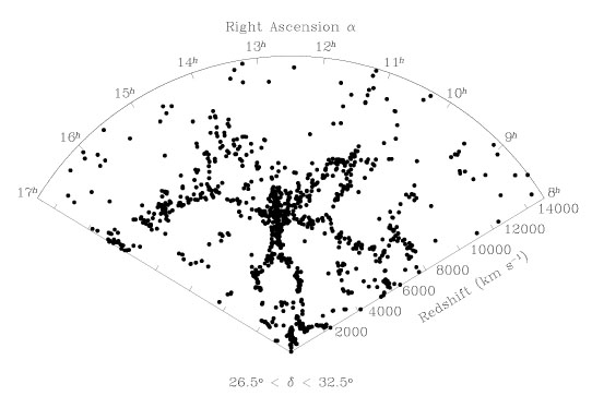
In 1986, de Lapparent, Geller & Huchra published their first
6° wide slice of a deeper extension of the original CfA
survey. The galaxy distribution in this two-dimensional slice is shown
in Fig. 3, from the data in
Huchra et al. (1990a).
Redshift is the radial coordinate, and right ascension is the angular
coordinate; declination is suppressed. This figure, which is often
compared to a slice through a network of bubbles, shows clearly that
voids like that in Boötes are ubiquitous, and that galaxies are
aligned along sheet-like structures.The structure stretching across
the entire slice at
cz 8000 km
s-1 has been called the Great Wall
(Geller & Huchra 1989
),
and is the largest structure known to exist (cf.,
Di Nella & Paturel 1994
).
Geller, Huchra, and collaborators are extending the
original CfA survey to
mZ = 15.5, over the full area covered by the
CGCG. The survey is nearing completion, and will contain roughly
15,500 galaxies at high latitudes and another 3000 in regions near the
Galactic plane. The median redshift is
7500 km
s-1. The results from this survey are reported in
de Lapparent et al.
(1986,
1988,
1989,
1991),
Huchra et al. (1990a),
Vogeley et al.
(1991,
1992,
1994),
Ramella et al. (1992),
and Park et al. (1994)
.
|
Figure 3. The galaxy distribution from the survey of de Lapparent et al. (1986), using the data of Huchra et al. (1990a). Redshift is plotted in the radial direction, and right ascension is the angular coordinate. Declination is suppressed. The prominent structure in the center of the figure is the Coma cluster. |
The Infrared Astronomical Satellite (IRAS) flew in 1983, and did a full-sky survey with ~ 1' resolution in four broad bands centered at 12, 25, 60, and 100µm. Because infrared radiation is not impeded by Galactic extinction, galaxy samples selected from the IRAS database are well-suited for full-sky redshift surveys. They do have the drawback, however, that early-type galaxies have very little dust or star formation, and thus are not represented in IRAS galaxy samples.
The first major redshift survey of IRAS galaxies (Soifer et al. 1987 ) consisted of the 324 galaxies with f60 > 5.4 Jy with |b| > 30° in the Northern sky. Strauss and collaborators carried out a survey covering 11.06 ster (88% of the sky, missing only regions at very low Galactic latitudes and areas not surveyed by IRAS) and including all 2658 galaxies to f60 = 1.936 Jy. Fisher et al. (1995) followed this up with a deeper survey over the same region of sky to f60 = 1.2 Jy, for a total of 5339 galaxies; redshifts are 99.6% complete. The median redshift of this survey is 5800 km s-1. Scientific results from this survey include Strauss et al. (1990, 1992a, b, c), Yahil et al. (1991) , Fisher et al. (1992, 1993, 1994a, b, c, 1995), Bouchet et al. (1993) , and Dekel et al. (1993) .
A parallel effort led by Rowan-Robinson consisted of a sparse sample of one in six IRAS galaxies to a flux limit of f60 = 0.6 Jy. The selection criteria differed in detail from the IRAS surveys mentioned before, and covered a solid angle of 10.3 ster with 2184 galaxies. This survey is deeper but sparser than the complete IRAS surveys, with a median redshift of 8400 km s-1. This survey is nicknamed QDOT, after the institutions of the investigators. Major papers include Rowan-Robinson et al. (1990) , Efstathiou et al. (1990) , Saunders et al. (1990) , Saunders et al. (1991) , Kaiser et al. (1991) , and Lawrence et al. (1994) .
Loveday et al. (1992a, b, 1995) have carried out a redshift survey following up the APM photometric survey of Maddox et al. (1990a, b, c). They measured redshifts for one in twenty of galaxies brighter than bJ = 17.15 over 1.3 steradians centered on the Southern Galactic Cap. The sample contains 1787 galaxies with a median redshift of 15,200 km s-1.
Although not a redshift survey itself, the effort of Hudson (1993a, b, 1994a, b) should also be mentioned. He calculated the redshift incompleteness (using the compilation of Huchra et al. 1992 ) of the UGC and ESO catalogs as a function of diameter and position on the sky, and statistically corrected the redshift maps accordingly, allowing him to recreate the full optical galaxy density field, which he used for comparison to peculiar velocity studies (Section 8.1).
There are also a number of redshift surveys in progress or in the advanced planning stages (see the volume edited by Maddox & Aragón-Salamanca 1995 for papers on these and other surveys in progress):
< - 2.5°)
they use the recently completed diameter-limited Extension to the
Southern Galaxy Catalog
(Corwin & Skiff 1994
).
The sample is limited by Galactic extinction to
|b| > 20°, covers 8.09 ster,
and contains 8457 galaxies, of which redshifts are available for
8286. The median redshift is 3900
km s-1. The sample and the resulting
galaxy distribution are presented in
Santiago et al. (1995a,
b)
and Santiago (1994)
.
15, 000 galaxies. A
parallel effort is using the
IRAS Faint Source Survey to push to 0.2 Jy at 60µm
over a much smaller area of sky (cf.
Lonsdale et al. 1990
).
The more ambitious surveys mentioned here are going deeper than existing catalogs of galaxies extend. Thus workers are being forced to define galaxy samples themselves. This turns out to be a boon (although a great deal more work) as now the galaxy selection criteria can be fine-tuned for the purposes of redshift survey work and large-scale structure studies. In addition, the modern automated methods of galaxy selection and photometry yield more reliable catalogs with much more robust magnitudes than those measured by eye. Two further redshift surveys in the advanced planning stages are discussed in a final concluding section (Section 9.7).
3.3. The Measurement of Galaxy Redshifts
The majority of the redshift surveys discussed above have redshifts
measured in the optical part of the spectrum. This is done typically
with telescopes of aperture between one and five meters, attached to
low- or medium resolution (R

 /
/
 ~ 1000) spectrographs. At much
higher resolution, one resolves the
internal motions of the galaxies themselves; at much lower resolution,
individual spectral features begin to blend with one another.
~ 1000) spectrographs. At much
higher resolution, one resolves the
internal motions of the galaxies themselves; at much lower resolution,
individual spectral features begin to blend with one another.
The optical spectra of the vast majority of galaxies fall into one of several types:
The measurement of redshifts of low-surface brightness galaxies is
always difficult. If the object is too faint to measure a continuum
with enough signal-to-noise ratio to detect absorption lines, one can
either "pray for H ", hoping
that an HII
region will fall on the slit, or observe these objects in the radio,
looking for 21 cm transition of HI; late-type
low-surface brightness galaxies are often rich in
HI, and surveys of these objects have been carried
out with radio telescopes
(Bothun et al. 1985
,
Schneider, Thuan, & Mangum 1992
).
", hoping
that an HII
region will fall on the slit, or observe these objects in the radio,
looking for 21 cm transition of HI; late-type
low-surface brightness galaxies are often rich in
HI, and surveys of these objects have been carried
out with radio telescopes
(Bothun et al. 1985
,
Schneider, Thuan, & Mangum 1992
).
The measurement of emission-line redshifts is straightforward, and is usually done by fitting multiple Gaussians to the lines that are seen. Absorption-line redshifts require more subtlety: the absorption lines are typically of lower signal-to-noise ratio, and the features that are seen often consist of blends of lines, making it impossible to assign the feature to a unique redshift. A redshift is measured by comparing the spectrum of the galaxy in question to that of a star of known (small) radial velocity, typically a K0-K3 giant taken with the same instrumental setup. Heuristically, one slides the spectrum of the stellar template back and forth until it matches the spectrum of the galaxy, the amount of the shift being a measure of the redshift. In practice, this is done by taking cross-correlating the spectra of the galaxy and the stellar template in either Fourier or real space, and fitting the peak with a smooth function (Sargent et al. 1977 ; Tonry & Davis 1979 ; Heavens 1993 ). Using such techniques redshifts of nearby galaxies are typically measured with ~ 50 km s-1 accuracy (e.g., Huchra et al. 1983 ).
In the days when blue-sensitive photographic plates were the detecting
element in spectrographs, spectra for redshifts of nearby galaxies
were often taken in the blue region of the spectrum covering the
region around 4000Å, in order to detect the Calcium H and K lines.
Modern CCD detectors are more sensitive in the red, and spectra are
typically taken centered on the 5175Å Mg b feature, or, for
galaxies that are likely to have strong emission lines, centered on
H and the
[NII] doublet at ~ 6550Å. CCD detectors on
most modern spectrographs have of the
order of 800 pixels along the dispersion direction, with roughly two
pixels per dispersion element, implying a spectral coverage of
2000Å for R = 1000. As CCDs get larger, it is becoming
possible to cover more of the visible part of the spectrum, and double
spectrographs which use a dichroic to split the light into red and
blue halves, each going to a separate camera, are now operating on the
Palomar 5m, Lick 3m, ARC 3.5m, Keck 10m, and other telescopes.
Most of the redshift surveys listed above have been carried out by observing one object at a time. However, now that multi-object spectrographs exist on many of the world's largest telescopes, it is possible to obtain spectra for many galaxies in a single exposure. In practice, the size of the telescope determines the faintness of the galaxies for which one can obtain redshifts in a reasonable exposure time, and this faintness limit in turn determines the mean number density of galaxies on the sky. Thus one designs a multi-object spectrograph with a number of fibers and field of view with these considerations in mind. This is the approach taken by the Kirshner et al. Las Campanas survey and the Sloan Digital Sky Survey (Section 9.7), among others.
Redshift surveys are also carried out in the radio, where one looks for the HI 21 cm line in emission. As elliptical galaxies tend to be gas-poor, such surveys are limited to later-type galaxies. The largest such redshift surveys have been done at Arecibo Observatory in Puerto Rico, and with the 140-foot and the late 300-foot telescopes at Green Bank, West Virginia. These surveys are carried out at much higher resolution than in the optical, typically R = 30, 000. Thus radio redshifts are typically measured to much higher accuracy than optical redshifts, with quoted errors of 5-10 km s-1. The combination of loss of sensitivity, and the fact that the 21 cm line is redshifted into an unprotected band, means that radio surveys are unable to probe redshifts much beyond 10,000 km s-1, although the Giant Metrewave Radio Telescope near Puna, India, will be able to get around these problems with its enormous collecting area and relative isolation. In some of the older HI redshift literature, the redshift was not defined by Eq. (8), but by

| (53) |
which agrees with Eq. (8) only for infinitesimal z. The reader of the older literature must be aware of this potential for confusion, although modern workers consistently use the "optical definition" of z, Eq. (8).
Redshifts are measured, by necessity, on a telescope attached to the
Earth. The Earth takes part in many motions: it is rotating on its own
axis (0.3 km s-1 at the equator), and it is orbiting around
the Sun (30 km s-1). For extragalactic work, the former
correction is negligible,
but redshifts are usually published with the correction to the
heliocentric frame. However, the Sun is in orbit around the center of
the Milky Way ( 225
km s-1), the Milky Way is falling towards
our nearest large companion, M31 at 119 km s-1
(Binney & Tremaine
1987),
and the whole Local Group of galaxies takes part in the
larger-scale velocity field which we will discuss in detail
below. Because motions on scales smaller than that of the Local Group
are very non-linear, we will not include them in our models, but
rather refer to redshifts relative to the barycenter of the Local
Group. Estimates for the correction from the heliocentric to Local
Group barycentric frame have been given by
Yahil, Tammann, &
Sandage (1977)
,
de Vaucouleurs, de Vaucouleurs, & Corwin (1976)
and Lynden-Bell & Lahav (1988)
.
These three determinations are consistent
with one another; for example, Yahil et al. quote the motion of the
sun relative to the barycenter as 307 km s-1 towards Galactic
coordinates l = 105°, b = - 7°.
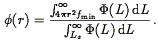
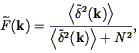
3.4. Determination of the Luminosity and Selection Functions
Redshift surveys have the property that the number density of sample
objects is a decreasing function of redshift. We quantify this in
terms of a selection function
 (r), defined as the
fraction of galaxies at distance r which meet the sample selection
criteria. In order to use the
galaxies in a sample as tracers of the general galaxy distribution, we
must correct for the fact that the galaxies represent an increasingly
smaller proportion of the parent population at larger and larger
distances. We do this by giving sample objects weights
proportional to 1/(r) in
order to account for the galaxies below
the flux limit at distance r. The selection function
is closely related to the luminosity function
(r), defined as the
fraction of galaxies at distance r which meet the sample selection
criteria. In order to use the
galaxies in a sample as tracers of the general galaxy distribution, we
must correct for the fact that the galaxies represent an increasingly
smaller proportion of the parent population at larger and larger
distances. We do this by giving sample objects weights
proportional to 1/(r) in
order to account for the galaxies below
the flux limit at distance r. The selection function
is closely related to the luminosity function
 (L), which
gives the number density of galaxies of luminosity L, per unit
luminosity. The relationship between
(r) and
(L) is most
easily seen in the case of a survey in which the sample is defined by
a minimum energy flux fmin; the derivation to follow
may be
trivially modified for a survey limited by apparent diameter or other
photometric quantity, or for direction-dependent selection (as in the
case of samples affected by Galactic extinction; cf.,
Santiago et al. 1995b
).
In the latter case, one generalizes the selection function to
a quantity depending on both distance and direction on the sky.
(L), which
gives the number density of galaxies of luminosity L, per unit
luminosity. The relationship between
(r) and
(L) is most
easily seen in the case of a survey in which the sample is defined by
a minimum energy flux fmin; the derivation to follow
may be
trivially modified for a survey limited by apparent diameter or other
photometric quantity, or for direction-dependent selection (as in the
case of samples affected by Galactic extinction; cf.,
Santiago et al. 1995b
).
In the latter case, one generalizes the selection function to
a quantity depending on both distance and direction on the sky.
The integral of (L) over
all L gives the total number density
of galaxies, n. In practice, the luminosity function is poorly
constrained at the faint end, and so we cut off the integral at a
lower limit
Ls 4
 rs2
fmin for some small rs
(typically 500 km s-1), and reject galaxies with lower
luminosities. At any distance r > rs, we
can only observe galaxies with luminosities greater than
rs2
fmin for some small rs
(typically 500 km s-1), and reject galaxies with lower
luminosities. At any distance r > rs, we
can only observe galaxies with luminosities greater than
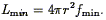
| (54) |
Consequently, the ratio of observable to total galaxies at distance r is
| (55) |
At distances closer than rs, we set
(r)
1. Note that
the luminosity function is a property of the galaxies themselves,
while the selection function depends on the photometric limits of the
sample in question.
The use of the selection function to weight galaxies in large-scale structure studies makes the assumption that the luminosity function is universal, independent of local density. This assumption means that galaxies of any luminosity are equally good tracers of the large-scale galaxy distribution (cf. Section 5.10), or equivalently, that that bivariate distribution of galaxies in position and luminosity is a separable function.
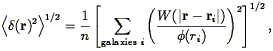
There are several methods for measuring the luminosity or selection function from redshift surveys. The simplest is called the 1 / Vmax method, due to Schmidt (1968) : the luminosity of a galaxy in the sample determines a maximum distance to which it could be placed and still remain within the sample:
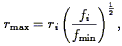
| (56) |
where ri and fi are the measured
distance and flux of the source. We can then define a maximum volume,
 rmax3/3, where
is the solid angle
covered by the survey. The estimator for the luminosity function is then
rmax3/3, where
is the solid angle
covered by the survey. The estimator for the luminosity function is then
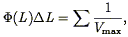
| (57) |
where the sum is over all galaxies with measured luminosities between
L and L +
L.
This method is easily generalized to the case of a variable
flux limit, caused, for example, by Galactic extinction. However, it
makes the assumption that the mean underlying number density of
galaxies is uniform, without any density inhomogeneities. This is a
dangerous assumption, for we shall see that the inhomogeneities can be
substantial.
There is an extensive literature of methods to derive selection
functions in density-independent ways
(Lynden-Bell 1971
,
Turner 1979
,
Kirshner et al. 1978,
Sandage, Tammann, & Yahil 1979
,
Davis & Huchra 1982
,
Nicoll & Segal 1982
,
Efstathiou, Ellis, & Peterson 1988
,
Choloniewski 1986
,
Binggeli et al. 1988,
and Yahil et al. 1991
).
We present here our own favorite, following the development of
Yahil et al. (1991)
.
We phrase the problem in terms of likelihoods: given
that a galaxy i is at distance ri, what is the
probability that it fall in the interval
L < Li < L + dL?
This probability is simply the luminosity function
(Li),
normalized by the integral over all luminosities it could have at that
distance, given the flux limit of the survey:
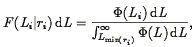
| (58) |
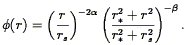
where Lmin(r) was defined in Eq. (54). Note that as written, F(Li| ri) is a probability density, per unit luminosity. It will be convenient to rephrase Eq. (58) in terms of the selection function:
| (59) |
where rmax was defined in Eq. (56). This is
the likelihood for a single galaxy, given the selection function; the
likelihood for the entire sample is then the product of F over all
the galaxies in the sample. We then solve for the selection function
by maximizing the likelihood with respect to the parameters
in terms of which we model
(r). Note
that we need not worry about the constant of proportionality in
Eq. (59), as it is independent of the selection
function itself, and therefore is irrelevant when maximizing with
respect to .
Note that the likelihood function is indeed independent of the underlying density distribution, as it is a conditional probability for the luminosities, given the distances to each object. In particular, this method is independent of the mean density of the sample, which drops out of the ratio in Eq. (58). Thus we need an independent way to define the mean density. Davis & Huchra (1982) discuss various methods for defining the mean density of a sample given the selection function. In general, the mean density is given by a weighted sum over the sample:
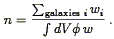
| (60) |
In the presence of density inhomogeneities, the variance in n is minimized with the weights:
| (61) |
where
| (62) |
is a measure of the density fluctuations on the scale of the survey.
Because of the presence of n in the expression for the weights, one
has to calculate n iteratively. In practice, one often uses the
simpler estimator, given by
wi = 1 /
(ri), thus:
| (63) |
In principle, one sums over all the galaxies of the survey, in which case V is the volume out to the most distant object of the sample. In practice, this would be horribly noisy, and one sums out to a radius beyond which the sample becomes so sparse that the shot noise of Eq. (63) dominates.
Given a value of n, one can define the luminosity function in terms of the selection function. One often sees the luminosity function expressed in logarithmic intervals of luminosity, so that:
| (64) |
How in practice does one maximize the likelihood with respect to an
unknown function? One approach is to use a parameterized form for the
selection function, and maximize with respect to those parameters
(Sandage et al. 1979,
Yahil et al. 1991
).
It is easier to work with a
parameterized form for rather
than because it is always
easier to differentiate than to integrate.
Yahil et al. (1991)
suggest a simple generic form for
with three parameters, which is
applicable to a variety of situations:
| (65) |
Alternatively, one can write the luminosity function in the form of a series of steps:

| (66) |
The steps Lk are typically logarithmically spaced, and
the aim is to solve for the parameters
k. The selection
function can then be written
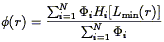
| (67) |
where
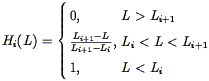
| (68) |
Setting the derivative of the likelihood function
(Eq. 58) with respect to the
i to zero yields
a series of implicit equations for the
's which are solved by iteration
(Nicoll & Segal 1982
;
Efstathiou et
al. 1988).
This method has two drawbacks
(Koranyi & Strauss 1994).
First, because the
luminosity function is taken to be constant over a finite interval,
the selection function has discontinuous first derivatives, and in
fact is biased upwards; this makes further analyses based on the
selection function misleading. This can be fixed by fitting a smooth
curve through the steps and calculating the selection function from
this. Alternatively, one can use a generalization of
Eq. (66), in which one linearly interpolates the
luminosity function between steps. Second and more serious, when the
number of steps becomes small, the luminosity function is biased
downwards, especially at the faint end, an effect which requires a
large number of steps (40 or more) to mitigate. We will discuss one
effect of this bias in Section 3.6.
Maximum-likelihood methods in general, and the ones we have described here in particular, have the disadvantage that there is no explicit measure of goodness-of-fit. Thus when fitting for a parameterized form, one can be sure to get the best values of the parameters out, but one can never know whether the form itself is adequate. Sandage et al. (1979) and Yahil et al. (1991) have developed a simple a posteriori method to test how well a given selection function fits the sample. One can compare the observed distribution of luminosities in a redshift sample with that expected, given the distances and a model for the luminosity function. Eq. (58) is the probability distribution function of luminosity for a galaxy at a given distance, with a sharp cutoff at Lmin(r). One can carry out this comparison for any well-defined subset of the data (defined by redshift, position on the sky, morphological type, local density, etc.) that does not have explicit selection on luminosity. Fig. 4 illustrates this for the IRAS 1.2 Jy survey: in each panel, the smooth curve is the predicted luminosity distribution, while the histogram is that observed; the agreement is excellent. The different panels show the luminosity distribution in different redshift shells, indicating that there are no systematic errors as a function of redshift. Actually, it remains unclear how useful this test is; experiments show that the luminosity function must be very seriously in error before this test shows disagreement between observed and predicted luminosity distributions.
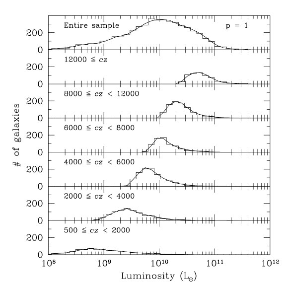
|
Figure 4. The luminosity distribution
(histogram) of the IRAS 1.2 Jy
sample in different redshift ranges, together with the predicted
distributions, given the luminosity function. The values of
|
As discussed in Section 3.1, the photometric data on which a redshift survey is based are not always of the highest quality. This has two effects: objects will be scattered in and out of the sample by flux errors, and errors in fluxes will cause luminosities to be in error. Because there are many more faint than bright galaxies, the net effect of errors is to cause a systematic over-estimation of luminosities. It is straightforward to show that constant fractional errors in the fluxes result in a derived luminosity function that is a convolution of the true underlying luminosity function with the flux error distribution. Monte-Carlo experiments by Santiago et al. (1995b) show that despite this effect, the density field derived from redshift survey data is quite robust to flux errors. That is, the bias in the selection function caused by flux errors is very nearly cancelled by the bias in galaxy counts caused by objects scattering across the flux limit. The density field is more robust than is the luminosity function itself to flux errors, as long as the selection function is measured from the same dataset.
A comprehensive review of determinations of the luminosity function is given in Binggeli et al. (1988), cf. Felten (1977) for earlier work. Modern determinations of the luminosity functions of galaxies in optically selected bands include Efstathiou et al. (1988), Loveday et al. (1992b, 1995), de Lapparent et al. (1989), and Marzke, Huchra, & Geller (1994) , while the IRAS luminosity function has been discussed by Saunders et al. (1990) , Yahil et al. (1991) , Spinoglio & Malkan 1989 , and Soifer et al. (1989) . The optical luminosity function is often fit to a form originally suggested by Schechter (1976) :
| (69) |
with free parameters and
L*; the sharp exponential cutoff
means that galaxies with luminosities well above L*
(the "knee"
of the luminosity function) are quite rare. The 60µm luminosity
function of IRAS galaxies does not show such a sharp cutoff, but
rather is well-fit by two power-laws (cf. Eq. 65); there is therefore a
substantial
population of ultraluminous IRAS galaxies, whose properties are the
subject of much research (e.g.,
Sanders et al. 1989).
This also means that the selection function of IRAS galaxies
is not as steep as that of optically selected galaxies, and thus
IRAS redshift surveys include a much more extensive tail of
high-redshift galaxies than does an optically selected sample with the
same median redshift (Figure 4 of
Santiago et al. 1995a).
3.5. Luminosity Functions: Scientific Results
The determination of the optical luminosity function of galaxies in optical bands has only been done adequately in the photographic B-band, in which the comprehensive galaxy catalogs have been compiled. Indeed, much remains to be learned about the distribution of galaxy properties in quantities other than luminosity. For example, Binggeli et al. (1988) stress that the luminosity function of galaxies is a strong function of galaxy morphology (cf. Loveday et al. 1992b , 1994), and although some work has been done on the diameter function of galaxies (Lahav et al. 1988; Maia & da Costa 1990; Hudson & Lynden-Bell 1991), the bivariate distribution of diameters and luminosities has barely been explored (Choloniewski 1985 ; Sodré & Lahav 1993). Even less is known about the bivariate distribution of luminosities and galaxy colors. Proper analyses of these basic properties of galaxies will require large samples of galaxies with excellent photometry in a variety of bands. This is one of the main scientific goals of the Sloan Digital Sky Survey. The galaxy luminosity function is a basic datum that any detailed model of galaxy formation must match; theoretical papers addressing this include White et al. (1987) , Schaeffer & Silk (1988) , White & Frenk (1991) , Cen & Ostriker (1992a) , Cole et al. (1994a), and White (1994) .
The measured luminosity function becomes very uncertain at the faint end (e.g., Efstathiou et al. 1988). The faint-end slope of the luminosity function has important ramifications for a number of issues in astrophysics. First, number counts of faint galaxies show an excess over the number predicted by simple extrapolation of the galaxy luminosity function today (Tyson 1988 ; Cowie et al. 1989 ; Maddox et al. 1990d ; Ellis 1993); if there is a population of galaxies that were bright in the past but whose surface brightnesses dimmed substantially as star formation ceased, they could be hidden today in the faint end of the luminosity function (McGaugh 1994 ). As photographic and CCD surveys push to ever lower surface brightness levels, new populations of galaxies are appearing (Bothun et al. 1987 ; Schombert & Bothun 1988 ; Schombert et al. 1992 ; Dalcanton 1994), including many galaxies of quite substantial luminosities.
Understanding the low-luminosity population is also important for understanding the evolution of metals (i.e., elements beyond Helium in the periodic table) in the universe. Cowie (1988) shows that the integrated surface brightness of galaxies in the sky is directly proportional to the total metal abundance:

| (70) |
where  Z is
the volume density of metals in the universe, and
Z is
the volume density of metals in the universe, and

 0 is the light emitted per unit
frequency per
unit mass of metals returned to the interstellar medium. Quantifying
the full galaxy population and therefore the total surface brightness
of the night sky due to galaxies
(Spinrad & Stone 1978
,
Toller 1990)
will thus give insights into the production of metals and the chemical
evolution of the universe.
0 is the light emitted per unit
frequency per
unit mass of metals returned to the interstellar medium. Quantifying
the full galaxy population and therefore the total surface brightness
of the night sky due to galaxies
(Spinrad & Stone 1978
,
Toller 1990)
will thus give insights into the production of metals and the chemical
evolution of the universe.
The numbers of low-luminosity galaxies is also vitally important for
quantifying the luminosity density of the universe. The total
emissivity of optical light per unit volume in the universe is given
by  L(L)dL,
which diverges if the faint-end logarithmic
slope of (L) is steeper
than = 2
(Eq. 69) (13).
We observe a dark night sky, which says that
the luminosity density of the universe does not in fact diverge at the
faint end, thus either the faint-end slope is somewhat shallower than
= 2, or there is a cut-off
at some point. The observational
situation is still very much in a state of flux; this is an active
area of research.
L(L)dL,
which diverges if the faint-end logarithmic
slope of (L) is steeper
than = 2
(Eq. 69) (13).
We observe a dark night sky, which says that
the luminosity density of the universe does not in fact diverge at the
faint end, thus either the faint-end slope is somewhat shallower than
= 2, or there is a cut-off
at some point. The observational
situation is still very much in a state of flux; this is an active
area of research.
The optical luminosity density of the universe can be turned into a
mass density of the stars if one assumes a mass-to-light ratio for the
stars. Alternatively,
Loveday et al. (1992b)
calculate the
mass-to-light ratio necessary to close the universe (i.e., such that
 0 = 1), given the
measured luminosity density, as
1580 ± 190h in solar units. For comparison, standard
spectral synthesis models give mass to blue luminosity ratios of 4 - 7.
0 = 1), given the
measured luminosity density, as
1580 ± 190h in solar units. For comparison, standard
spectral synthesis models give mass to blue luminosity ratios of 4 - 7.
The recent interest in low-luminosity and low surface brightness galaxies reminds us that the galaxy samples which form our basis for redshift surveys are likely to suffer from incompleteness (Disney 1976 ; McGaugh 1994). Even a survey limited at bright magnitudes or large diameters will miss a population of low-surface brightness galaxies, some of which are quite luminous (Bothun et al. 1987), although the numbers of luminous low-surface brightness galaxies seems to be quite small. There is also a bias against finding compact galaxies of very high surface brightness; these galaxies can be difficult to distinguish from stars (which are much more numerous than galaxies at all Galactic latitudes until one pushes to 22nd magnitude and fainter) and thus will be missed from the survey. The extreme examples of compact galaxies are the quasars: 3C 273 is bright enough to satisfy the selection criteria of the CfA redshift survey, but appears absolutely stellar on photographic plates; the host galaxy is apparent only with deep exposures under superb conditions (Hutchings & Neff 1991 ; Bahcall, Kirhakos, & Schneider 1994).
3.6. Testing the Hubble Law with Redshift Surveys
The observational evidence for the Hubble law (Eq. 1) for nearby galaxies is mostly based on distance indicator relations for individual galaxies. These usually take the form of standard candles, whereby the absolute luminosity of the galaxy or some well-defined part of it (e.g., Cepheid variables) are assumed to be known a priori (Section 6.1). Observation of its apparent luminosity gives the distance via the inverse-square law. This can then be compared with the redshift as a check of Eq. (1). The history of this approach is summarized in Chapter 5 of Peebles (1993) ; see Lauer & Postman (1992) for a recent test of the Hubble law. There has been no strong evidence for deviations from Eq. (1) beyond that expected from peculiar motions (Eq. 2). Nevertheless, one could imagine generalizing Eq. (1) to the form

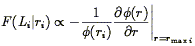
| (71) |
Segal et al. (1993, and references therein) suggest a so-called Chronometric Cosmology, in which p = 2 at low redshifts. Segal et al. (1993) suggest an intriguing measure of p from redshift surveys. Rather than using distance indicators to measure the distances to individual galaxies, one can use the luminosity function of galaxies as a distance indicator, assuming the luminosity function to be universal. In fact, luminosity function fitting has been used in the past to measure distances to galaxy clusters (Schechter 1976 ; Schechter & Press 1976 ; Gudehus 1989); here we wish to use it to test the Hubble law. Imagine that one interprets the results of a redshift survey using Eq. (71) with the incorrect value for p. One would expect that the luminosity function determined from subsets of the sample in different redshift ranges would not be consistent with one another; agreement would be found only for the correct value for p, and this then has the potential for distinguishing between different cosmological models. Segal et al. (1993) use the IRAS 1.936 Jy redshift survey (Strauss et al. 1992b) to claim that the data are consistent with p = 2 and inconsistent with the conventional p = 1. However, the luminosity function in different redshift shells is a much less powerful statistic than Segal et al. claim. In the limit of thin redshift shells, it is just measuring the flux distribution of the sample, and in any redshift survey, the majority of the sources are close to the flux limit, independent of cosmology. Koranyi & Strauss (1994) show that this distribution is almost independent of p, if one self-consistently derives the luminosity function from the sample for each value of p. Moreover, because Segal et al. use the step-wise luminosity function method described above, their luminosity function is systematically in error, the error being worse for smaller p than for larger. Therefore, their luminosity function for p = 2 is a better fit to the data than is p = 1, and they erroneously conclude that the Hubble law is ruled out by the data.
Although the luminosity function is a poor discriminant of models, one
can still use redshift surveys alone to put constraints on p. In a
homogeneous universe, the number of galaxies in a redshift survey with
redshift between r and r + r is
n(r)
r2r.
The upper panel of Fig. 5 compares the observed
histogram of redshifts of galaxies in logarithmic bins from the 1.2 Jy
IRAS survey with that predicted for p = 1, 2, and 3. Note
that
this is an independent test from that of the density-independent
luminosity function diagnostic described above. In the p
 1 models,
the predicted and observed redshift histograms are in bad
disagreement. The resulting density relative to the mean in shells
(the ratio of the histogram to the smooth curves) is
shown in the lower panel. In the standard cosmology, the almost
full-sky coverage of the IRAS survey averages over most density
structures, meaning that the sample is close to mean density at all
redshifts (cf.
de Lapparent et
al. 1988),
although the overdensity
associated with the Local Supercluster is apparent at
cz = 1000 km s-1. However, for the
p = 2 and p = 3 cosmologies, one must
argue that the Local Group lies in the middle of a void, surrounded by
a vast spherical shell at the mean density between 4000 and 10,000 km
s-1, which is surrounded by another spherical void extending
to the horizon.
1 models,
the predicted and observed redshift histograms are in bad
disagreement. The resulting density relative to the mean in shells
(the ratio of the histogram to the smooth curves) is
shown in the lower panel. In the standard cosmology, the almost
full-sky coverage of the IRAS survey averages over most density
structures, meaning that the sample is close to mean density at all
redshifts (cf.
de Lapparent et
al. 1988),
although the overdensity
associated with the Local Supercluster is apparent at
cz = 1000 km s-1. However, for the
p = 2 and p = 3 cosmologies, one must
argue that the Local Group lies in the middle of a void, surrounded by
a vast spherical shell at the mean density between 4000 and 10,000 km
s-1, which is surrounded by another spherical void extending
to the horizon.

|
Figure 5. The upper panel shows the redshift distribution of the IRAS 1.2 Jy sample, together with the expected distributions in a homogeneous universe, for various redshift-distance relations. The lower panel shows the ratio between the observed and expected distributions, which is the radial density field. Note that p = 1 (the Hubble Law) remains close to the mean density at all radii. |
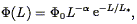
3.7. The Smoothed Density Field
We have seen above that the number density of galaxies in a flux
limited redshift survey is a decreasing function of distance. We
correct for this by assigning each galaxy a weight given by the
inverse of the selection function
(r). In order to define the
extent of the structures traced by the galaxies, we would like to
define a continuous density field. This is done by smoothing (cf.,
Eq. 24):
| (72) |
where the window function W is normalized to unit integral:
| (73) |
Common window functions used are top-hat, parabolic, and Gaussian:
| (74) |
All that remains is to choose a smoothing radius
rsmooth. Because the mean interparticle spacing of a
redshift survey is an increasing function of distance from the origin
(indeed, it is given by
[4
n (r) /
3]-1/3) a
smoothing length which shows full detail at small distances will
contain increasingly fewer particles at larger distances, with
corresponding ever-increasing shot noise. For this reason, it is
common to choose a smoothing length which grows with radius,
proportional to the mean interparticle spacing. This has the
disadvantage of not being amenable to Fourier Transform techniques for
carrying out the smoothing in Eq. (72); more
important, the smoothed density field has different statistical
properties at low and high redshift. Nevertheless, it is useful for
qualitative and cosmographical description of the structures that are
seen, and in some sense shows the maximum amount of information in the
redshift survey.
The smoothed density field will be subject to errors from a variety of sources. These include:
| (75) |
because the mean value of
is zero by definition. There is a
further contribution to the shot noise in the mass density
field which depends on the variance in the mass-to-light ratio of
galaxies, but this term is important only for nearby galaxies in
typical redshift surveys, simply because 1 /
grows so quickly
(cf. Appendix A of
Strauss et al. 1992c).
One can filter the data to minimize the shot noise. The Wiener Filter
(cf. Press et al. 1992
,
Section 13.3) minimizes the variance
between the measured and true density fields. Let
(r) be
the true underlying fractional density field of galaxies, and let
 (r) be the measured
density field, with shot noise N included:
(r) be the measured
density field, with shot noise N included:
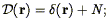
| (76) |
We assume for simplicity that the shot noise is independent of
position. Let us
define a filter F such that the difference between the filtered
density field
F and the true
density field is
minimized. In practice, we will work with Fourier Transforms, and
write:

| (77) |
by Parseval's Theorem. Substituting in Eq. (76)
and minimizing with respect to the unknown function
 (k), one finds the
Wiener filter:
(k), one finds the
Wiener filter:
| (78) |
where < 2(k)> is proportional to the power
spectrum P(k) of the
underlying density field
(14)
The Wiener filter requires a model for the
underlying power spectrum. We will discuss methods for estimating the
power spectrum from redshift survey data in
Section 5.3. Note that the Wiener filter
is defined in
k-space, because in real space, the values of
(r) at different
r are correlated. Indeed, the Wiener filter can be derived in real
space, in which case it is a matrix which takes this correlation
directly into account
(Zaroubi et al. 1994).
The number of elements in
the matrix is the square of the number of points at which one wishes
to define the density field, which becomes a very non-trivial
computational problem.
2(k)> is proportional to the power
spectrum P(k) of the
underlying density field
(14)
The Wiener filter requires a model for the
underlying power spectrum. We will discuss methods for estimating the
power spectrum from redshift survey data in
Section 5.3. Note that the Wiener filter
is defined in
k-space, because in real space, the values of
(r) at different
r are correlated. Indeed, the Wiener filter can be derived in real
space, in which case it is a matrix which takes this correlation
directly into account
(Zaroubi et al. 1994).
The number of elements in
the matrix is the square of the number of points at which one wishes
to define the density field, which becomes a very non-trivial
computational problem.
In a flux-limited redshift survey with a constant smoothing length, the noise term is an increasing function of r. In this case, one can either apply a Wiener filter in r space, as described above, or define a series of Wiener-filtered density fields at a range of values of N2, and interpolate between these at each point.
The Wiener filter approaches unity when the signal-to-noise ratio is high. At low signal-to-noise ratio, it approaches zero; when there is no information on the underlying density field, the filter returns the most likely value for the density, namely its mean. Thus the Wiener filter has the disadvantage of biasing the contrast in the density field downward. The expectation value of the square of the filtered field is
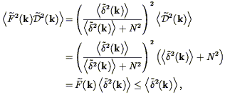
| (79) |
because
(k)
1 always. For comparison, the
expectation value of the square of the unfiltered field is
<2(k)> + N2
P(k). Thus the
Wiener
filter over-corrects the density field for shot noise. In the
case of a redshift survey for a constant smoothing length, the
signal-to-noise ratio is a decreasing function of r, and thus the
contrast of structures decreases with r, just as we had in the
variable smoothing mentioned above. Thus the Wiener filter offers a
natural way to invoke variable smoothing. For some problems, however,
this lack of statistical similarity between the nearby and far-away
parts of a redshift survey can be a drawback. In this case, one can
define an alternative filter, the power-preserving filter
(Yahil et al. 1994):
| (80) |
just the square root of the Wiener filter. This is just one of a
entire family of generalizations of the Wiener filter, as discussed
in, e.g.,
Andrews & Hunt
(1977) .
If we substitute the power-preserving filter into Eq. (79), we find
<FPP2(k)
 2(k)> =
<2(k)>, thus
the name power-preserving. Of course, this filter does not share the
minimum variance property of the Wiener filter, but it is easy to show
that for signal-to-noise ratios greater than one, the root-mean-square
difference between the filtered and true density fields is at most
10% larger for the power-preserving filter than for the Wiener
filter. As with the Wiener filter, Eq. (80) only holds
when the noise is independent of position;
Yahil et al. (1994)
interpolate between maps filtered with Eq. (80) at different
noise levels for the flux-limited case of noise increasing as a
function of distance.
2(k)> =
<2(k)>, thus
the name power-preserving. Of course, this filter does not share the
minimum variance property of the Wiener filter, but it is easy to show
that for signal-to-noise ratios greater than one, the root-mean-square
difference between the filtered and true density fields is at most
10% larger for the power-preserving filter than for the Wiener
filter. As with the Wiener filter, Eq. (80) only holds
when the noise is independent of position;
Yahil et al. (1994)
interpolate between maps filtered with Eq. (80) at different
noise levels for the flux-limited case of noise increasing as a
function of distance.
Although the power-preserving filter indeed preserves the second moment of the density distribution function, it does not do a good job of preserving higher-order moments at low signal-to-noise ratio (in particular, the skewness gets exaggerated), with the consequence that the filtered maps show sharper peaks in regions of low signal-to-noise ratio than in high. Work is ongoing to quantify this effect and correct for it.
3.8. Filling in the Galactic Plane
With the advent of galaxy surveys covering all of the sky outside of the Galactic plane, there has been a great deal of recent work expended on "finishing the job", that is, either extrapolating the density field at high latitudes to lower latitudes, or actually surveying in the zone of avoidance itself (Balkowski & Kraan-Korteweg 1994). There are two strong motivations for this. The first of these is cosmography: We would like to have a complete map of the structures of the local universe. The two largest superclusters in our immediate neighborhood, the Pisces-Perseus Supercluster and the Hydra-Centaurus Supercluster, both lie at low Galactic latitudes, and in both cases, there are overdensities on the opposite side of the plane (Camelopardalis and Pavo-Indus-Telescopium, respectively) to which they are plausibly physically connected.
The second reason for mapping the galaxy distribution at low
latitudes is for dynamical studies. Peculiar velocities and densities
are related in linear theory by Eq. (33); if we wish
to use this equation as a test of gravitational instability theory or to
measure 0, we
need as complete a map of the density field as possible.
Simply leaving unsurveyed regions unfilled causes systematic errors
in any dynamical modeling. The absence of galaxies does not
correspond to absence of structure; indeed, the unfilled regions will
act as a void with negative ,
from which
Eq. (33) predicts a systematic outflow. Filling the
unfilled regions of a survey with the average density of galaxies
corrects for this. The next order of approximation involves
interpolating the density field from higher-latitude regions. The
IRAS 1.936 Jy redshift survey has a low-latitude excluded zone that
is only 10° wide; for this,
Yahil et al. (1991)
advocate a
linear interpolation of the density field across the Galactic plane.
Lynden-Bell, Lahav,
& Burstein (1989)
have a 30° wide excluded
zone at low Galactic latitudes in their survey of optically selected
galaxies, and an additional 15° wide zone in the gap between
the areas of sky covered by the UGC and ESO catalogs. They use a
cloning procedure, in which galaxies are duplicated from adjacent
high-latitude regions into the excluded zones. A more elaborate
interpolation scheme was used by
Scharf et al. (1992)
who expanded the
angular distribution of IRAS galaxies in spherical harmonics, and
extrapolated them into the excluded zone. They found a
prominent overdensity in Puppis (which had been recognized
independently by
Kraan-Korteweg &
Huchtmeier 1992
and Yamada et
al. 1993 ),
which
Lahav et al. (1993b)
was able to show was a poor cluster at roughly the distance of Virgo.
Lahav et al. (1994)
advocate filtering the spherical harmonics with a Weiner filter to
reduce the noise; they show with N-body simulations that the
resulting reconstruction is quite robust for excluded zones less than
30° wide.
The observed velocity field at high latitudes depends on the density field at low latitudes. Using a density field reconstruction called POTENT (Section 7.5), Kolatt, Dekel, & Lahav (1995) have reconstructed the velocity field in the Zone of Avoidance. We will compare the results of this reconstruction to the density field of galaxies in Section 8.
An alternative approach to the various interpolation schemes discussed here is to survey the low-latitude sky directly. It is difficult to do quantitative work here, as the extinction is large and very variable. In regions that the extinction is not too strong (say, less than AB = 0.5 mag), one can correct for extinction statistically in the selection function, following the methods of Santiago et al. (1995b) ; the fewer galaxies in regions of high extinction are simply given greater weight to compensate. However, this process introduces a much larger shot noise. Various ongoing low-latitude searches for galaxies in the optical bands, and redshift surveys thereof, are summarized in the volume edited by Balkowski & Kraan-Korteweg (1994) .
One can also select galaxies in wavebands that are less affected than the optical by Galactic extinction. Galaxy catalogs selected at 60µm from the IRAS database have been used for redshift survey work. The principal limitations here are that any infrared color scheme that selects galaxies from stars and other Galactic objects becomes severely contaminated at low Galactic latitudes by emission nebulae and infrared cirrus (which has the same infrared colors as quiescent galaxies). At very low Galactic latitudes, the very high source density starts causing systematic errors in the IRAS fluxes. Finally, it becomes increasingly difficult to optically identify the galaxies in order to obtain redshifts when the optical extinction becomes too high. Despite these problems, the redshift surveys of Strauss et al. (1992b) , Fisher et al. (1995) , and Lawrence et al. (1994) extend down to within 5° of the Galactic plane. Low-latitude galaxy catalogs selected from the IRAS survey have also been published by Ichikawa & Nishida (1989) and Yamada et al. (1993) .
Neutral hydrogen 21 cm emission is also unaffected by Galactic extinction. Lu et al. (1990) have done HI surveys of IRAS sources, although Strauss et al. (1990) show that optical surveys are more efficient. But 21 cm surveys can also be done blindly, independent of any other catalog. Kerr & Henning (1987) used the late Green Bank 300 ft telescope to point to 1900 points; they discovered 16 previously uncatalogued galaxies. Kraan-Korteweg et al. (1994b) announce the discovery in HI of a new member of the group of which Maffei 1, Maffei 2, and IC 342 is a part. This is the first published result of a dedicated survey of the Northern Galactic plane (|b| < 5°) with the 25m Dwingeloo radio telescope, which is surveying out to a redshift of 4000 km s-1 with a resolution of 4 km s-1 and a beam size of 0.5° (FWHM).
Sky surveys at K band (2.2µm) are planned by both American and European teams. The extinction in this waveband is appreciably smaller than that in the optical bands, meaning that galaxy catalogs selected from this database will be able to penetrate to much lower Galactic latitudes. The Two Micron All Sky Survey (2MASS; Kleinmann 1992) will indeed cover the entire sky, and thus the galaxy sample selected from this survey will be ideal for measuring the dipole moment of the galaxy distribution (cf., Section 5.7). The Deep Extragalactic Near Infrared Survey (DENIS; Deul 1992), is planned only for the Southern Hemisphere, but will have superior angular resolution to the 2MASS survey.
13 Note that some workers use the
luminosity function per unit log luminosity, for which the
definition of differs by
unity from that here. See Eq. (64).
Back.
14 Eq. (78) holds only in the situation in which the noise is assumed independent of position. In the more realistic case of radially dependent noise, Eq. (78) generalizes to a two-dimensional matrix; cf., Fisher et al. (1995) for details. Back.
 2 / dof given
in each panel refer to the difference between the
two curves, with errors given by Poisson statistics.
2 / dof given
in each panel refer to the difference between the
two curves, with errors given by Poisson statistics.