3.2. Witten strings

The first model giving rise to scalar superconductivity in strings was proposed by Witten [1985]. His is a toy Abelian U(1) × U(1) model, in which two complex scalar fields, together with their associated gauge vector fields, interact through a term in the potential. In a way analogous to the structureless strings, one of the U(1) gauge groups is broken to produce standard strings. The other U(1) factor is the responsible for the current-carrying capabilities of the defect.

So, we now add a new set of terms, corresponding to a new complex scalar field , to the Lagrangian of Eq. (17). This new scalar field will be coupled to the also new vector field A⁽⁾_µ (eventually the photon field), with coupling constant e (e² ~ 1/137). The extra Lagrangian for the current is

(20)

with the additional interaction potential

(21)

and where, as usual, D_µ = (_µ + i e A⁽⁾_µ) and F⁽⁾_µ = _µ A⁽⁾ - A⁽⁾_µ. Remark that the complete potential term of the full theory under consideration now is the sum of Eq. (21) and the potential term of Eq. (17). The first thing one does, then, is to try and find the minimum of this full potential V(, ). It turns out that, provided the parameters are chosen as ² > v² and f²v⁴ < 1/8 ⁴, one gets the minimum of the potential for || = and || = 0. In particular we have V(|| = , || = 0) < V(|| = 0, || 0) and the group U(1) associated with A⁽⁾_µ remains unbroken. In the case of electromagnetism, this tells us that outside of the core, where the Higgs field takes on its true vacuum value || = , electromagnetism remains a symmetry of the theory, in agreement with the standard model. Hence, there exists a solution where (, A⁽⁾_µ) result in the Nielsen-Olesen vortex and where the new fields (, A⁽⁾_µ) vanish.

This is ok for the exterior region of the string, where the Higgs field attains its true vacuum. However, inside the core we have || = 0 and the full potential reduces to

(22)

Here, a vanishing is not the value that minimizes the potential inside the string core. On the contrary, within the string the value || = [2f / ]^1/2 v 0 is favored. Thus, a certain nonvanishing amplitude for this new field exists in the center of the string and slowly decreases towards the exterior, as it should to match the solution we wrote in the previous paragraph. In sum, the conditions in the core favor the formation of a -condensate. In a way analogous to what we saw for the Nielsen-Olesen vortex, now the new gauge group U(1), associated with A⁽⁾_µ, is broken. Then, it was = ||eⁱ and now the phase (t, z) is an additional internal degree of freedom of the theory: the Goldstone boson carrying U(1) charge (eventually, electric charge) up and down the string.

Let us now concentrate on the currents and field profiles. For the new local group U(1), the current can be computed as

(23)

Given the form for the `current carrier' field we get

(24)

From the classical Euler-Lagrange equation for , J^µ is conserved and well-defined even in the global or neutral case (i.e., when the coupling e = 0).

Now, let us recall the symmetry of the problem under consideration. The string is taken along the vertical z-axis and we are studying a stationary flow of current. Hence, the current J^µ cannot depend on internal coordinates a = t, z (by `internal' one generally means internal to the worldsheet of the string).

Conventionally, one takes the phase varying linearly with time and position along the string = t - k z and solves the full set of Euler-Lagrange equations, as in Peter [1992]. In so doing, one can write, along the core, J^a = -||² P^a and, in turn, P_a(r) = P_a(0) P(r) for each one of the internal coordinates, this way separating the value at the origin of the configuration from a common (for both coordinates) r-dependent solution P with the condition P(0) = 1. In this way, one can define the parameter w (do not confuse with ) such that w = P_z²(0) - P_t²(0) or, equivalently, P^a P_a = wP². Then the current satisfies J^aJ_a = ||⁴ w P².

The parameter w is important because from its sign one can know in which one of a set of qualitatively different regimes we are working. Actually, w leads to the following classification [Carter, 1997]

(25)

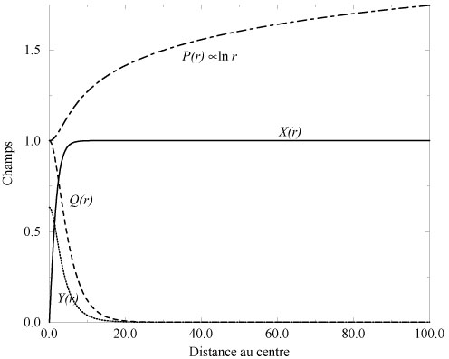
From the solution of the field equations one gets the standard logarithmic behavior for P_z = _z + e A_z⁽⁾ ln(r) far from the (long) string. This is the expected logarithmic divergence of the electromagnetic potential around an infinite current-carrier wire with `dc' current I that gives rise to a magnetic field B⁽⁾ 1/r (see Figure 1.7).

Figure 1.7. Profiles for the different fields around a conducting cosmic strings [Peter, 1992]. The figure shows the Higgs field (noted with the rescaled function X(r)), exactly as in the left panel of Figure 1.6. The profile Q(r) is essentially (the -component of) the gauge vector field A()µ, whose gradient helps in canceling the otherwise divergent energy density of the (global) string and concentrates the energy of the configuration inside a narrow core, as in the right panel of Figure 1.6. The profile Y(r) is a rescaled function for the amplitude of the current-carrier field . Its form shows clearly the existence of a boson condensate in the core of the string, signaling the flow of a current along the string. Finally, P(r) is essentially the electromagnetic field Az() with its standard logarithmic divergence.