1.2. Density estimates in the exploration and presentation of data

A very natural use of density estimates is in the informal investigation of the properties of a given set of data. Density estimates can give valuable indication of such features as skewness and multimodality in the data. In some cases they will yield conclusions that may then be regarded as self-evidently true, while in others all they will do is to point the way to further analysis and/or data collection.

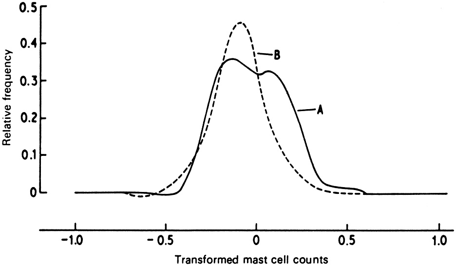
An example is given in Fig. 1.1. The curves shown in this figure were constructed by Emery and Carpenter (1974) in the course of a study of sudden infant death syndrome (also called `cot death' or `crib death'). The curve A is constructed from a particular observation, the degranulated mast cell count, made on each of 95 infants who died suddenly and apparently unaccountably, while the cases used to construct curve B were a control sample of 76 infants who died of known causes that would not affect the degranulated mast cell count. The investigators concluded tentatively from the density estimates that the density underlying the sudden infant death cases might be a mixture of the control density with a smaller proportion of a contaminating density of higher mean. Thus it appeared that in a minority (perhaps a quarter to a third) of the sudden deaths, the degranulated mast cell count was exceptionally high. In this example the conclusions could only be regarded as a cue for further clinical investigation.

Fig. 1.1 Density estimates constructed from transformed and corrected degranulated mast cell counts observed in a cot death study. (A, Unexpected deaths; B, Hospital deaths.) After Emery and Carpenter (1974) with the permission of the Canadian Foundation for the Study of Infant Deaths. This version reproduced from Silverman (1981a) with the permission of John Wiley & Sons Ltd.

Another example is given in Fig. 1.2. The data from which this figure was constructed were collected in an engineering experiment described by Bowyer (1980). The height of a steel surface above an arbitrary level was observed at about 15 000 points. The figure gives a density estimate constructed from the observed heights. It is clear from the figure that the distribution of height is skew and has a long lower tail. The tails of the distribution are particularly important to the engineer, because the upper tail represents the part of the surface which might come into contact with other surfaces, while the lower tail represents hollows where fatigue cracks can start and also where lubricant might gather. The non-normality of the density in Fig. 1.2 casts doubt on the Gaussian models typically used to model these surfaces, since these models would lead to a normal distribution of height. Models which allow a skew distribution of height would be more appropriate, and one such class of models was suggested for this data set by Adler and Firman (1981).

Fig. 1.2 Density estimate constructed from observations of the height of a steel surface. After Silverman (1980) with the permission of Academic Press, Inc. This version reproduced from Silverman (1981a) with the permission of John Wiley & Sons Ltd.

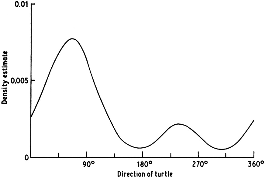
A third example is given in Fig. 1.3. The data used to construct this curve are a standard directional data set and consist of the directions in which each of 76 turtles was observed to swim when released. It is clear that most of the turtles show a preference for swimming approximately in the 60° direction, while a small proportion prefer exactly the opposite direction. Although further statistical modelling of these data is possible (see Mardia 1972) the density estimate really gives all the useful conclusions to be drawn from the data set.

Fig. 1.3 Density estimate constructed from turtle data. After Silverman (1978a) with the permission of the Biometrika Trustees. This version reproduced from Silverman (1981a) with the permission of John Wiley & Sons Ltd.

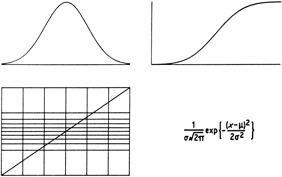
An important aspect of statistics, often neglected nowadays, is the presentation of data back to the client in order to provide explanation and illustration of conclusions that may possibly have been obtained by other means. Density estimates are ideal for this purpose, for the simple reason that they are fairly easily comprehensible to non-mathematicians. Even those statisticians who are sceptical about estimating densities would no doubt explain a normal distribution by drawing a bell-shaped curve rather than by one of the other methods illustrated in Fig. 1.4. In all the examples given in this section, the density estimates are as valuable for explaining conclusions as for drawing these conclusions in the first place. More examples illustrating the use of density estimates for exploratory and presentational purposes, including the important case of bivariate data, will be given in later chapters.

Fig. 1.4 Four ways of explaining the normal distribution: a graph of the density function; a graph of the cumulative distribution function; a straight line on probability paper, the formula for the density function.