Annu. Rev. Astron. Astrophys. 1994. 32: 319-70 Copyright © 1994 by Annual Reviews. All rights reserved

3.3. The Observed Power Spectrum

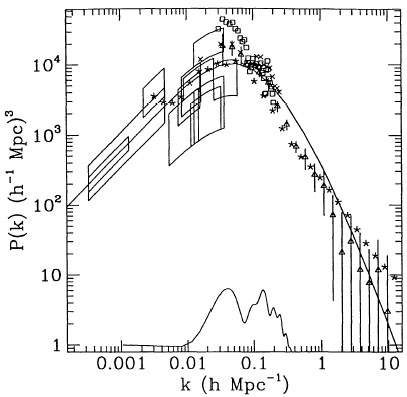
In this section, we consider the current status of measurements of the matter power spectrum (see Peacock 1991, Peacock & Dodds 1994), and the radiation power spectrum (see Bond 1993) in the context of inflation (see Liddle & Lyth 1993). In Figure 3 we compare the radiation power spectrum with the matter power spectrum measured by IRAS-selected galaxies (Fisher et al 1993, Feldman et al 1994), the CfA redshift survey (Vogeley et al 1992), and the APM galaxy survey (Baugh & Efstathiou 1993a, b).

Figure 3. The CDM matter power spectrum on a range of scales as inferred from CMB and LSS data. The solid line is CDM normalized to COBE. Stars, crosses, squares, and triangles are the APM, CfA, IRAS-QDOT, and IRAS-1.2Jy surveys respectively, with IRAS surveys scaled to 8DM = 1. Apart from scaling the IRAS surveys, we have avoided complicated issues related to normalization and redshift corrections. We show error bars on the IRAS-1.2Jy survey to indicate the approximate accuracy involved. The boxes are ± 1 values of the matter power spectrum inferred from CMB measurements assuming CDM with B = 0.06, with the horizontal extent taken to be between the half-peak points of the window functions for each experiment. From left to right the experiments are COBE, FIRS, Tenerife. SP91-13pt, Saskatoon, Python, ARGO, MSAM2, MAX-GUM & MAX-MuP, MSAM3. The radiation power spectrum for CDM assuming B = 0.06 is shown at the bottom.

Since one cannot make a theory-independent extrapolation from the radiation power spectrum (probed by CMB measurements) to the matter power spectrum (probed by large-scale structure work) in the following, we will assume CDM and write the matter power spectrum as

(24)

where A is as in (12) and T_m is a matter transfer function (see Equation 20), not to be confused with T(k). The change in units and the index of the power law from k⁰ to k¹ is a matter of convention. We follow the usual convention in large-scale structure (LSS) work that a "flat" spectrum has P_mat(k) k (see Liddle & Lyth 1993 for more discussion on the various definitions of power spectra) and work in units of h^-1 Mpc. To convert from our normalization to that of the bias or ₈ conventionally used in LSS work, see Equation (19); note that this conversion is senstive to any variation in the theory. The large-scale structure and CMB data are shown in Figure 3.

For the CMB anisotropy measurements, we have chosen some recent experiments for which we could estimate the best-fit normalization. Specifically, we show results from COBE (Smoot et al 1991, 1992; Wright et al 1994a), FIRS/MIT (Page et al 1990; Ganga et al 1993; Bond 1993, 1994), Tenerife (Davies et al 1992, Watson et al 1992, Hancock et al 1994), Python (Dragovan et al 1994), ARGO (de Bernardis et al 1993, 1994), SP91/ACME (13-point) (Schuster et al 1993), Saskatoon (Wollack et al 1993), MAX [MuP (Meinhold et al 1993) and GUM (Devlin et al 1993, Gundersen et al 1993)], and MSAM (Cheng et al 1994). We have concentrated here on those experiments that quote a detection, leaving out those that give only upper limits, e.g. Relikt (Klypin et al 1992), 19.2 GHz (Boughn et al 1992), SP89 (Meinhold & Lubin 1991), SP91-9pt (Gaier et al 1992), ULISSE (de Bernardis et al 1992), White Dish (Tucker et al 1993), OVRO (Readhead et al 1989, Myers et al 1993), and VLA (Fomalont et al 1993). Note we have also avoided complicated issues involving redshift space corrections (e.g. Kaiser 1987) to the large-scale structure data.

The P_mat(k) inferred from CMB anisotropies depends on the assumed theory (₀ for example shifts the correspondence between and k, and shifts the amplitude for a given T / T). Consequently, the boxes in Figure 3 would have to be redrawn for each theory.

In addition to the survey data shown in Figure 3, there is information on large-scale flows (e.g. Kashlinsky & Jones 1991). Bertschinger et al (1990a) estimated the 3-D velocity dispersion of galaxies within spheres of radius 40 h^-1 Mpc and 60 h^-1 Mpc. After smoothing with a Gaussian filter on 12 h^-1 Mpc scales they found _v(60) = 327 ± 82 km s^-1 and _v(40) = 388 ± 67 km s^-1. The unbiased CDM estimate for these quantities are 224 km s^-1 and 287 km s^-1 respectively. Translating this information into the power on scales of 40 h^-1 Mpc and 60 h^-1 Mpc gives roughly ₈ 1.15 (Efstathiou et al 1992).

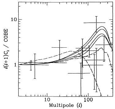
One can also consider the CMB data independently of theories of structure formation. In Figure 4, we show the current situation with regard to experiments that have quoted detections on degree scales or larger. We plot the normalization which, for an n = 1 power spectrum, would reproduce the quoted T / T_rms for each experiment. If there is a Doppler peak in the power spectrum on degree scales, then this would show up as a higher required normalization for a flat spectrum to fit the data. All of these points should be interpreted as approximations to the results of a full analysis.

Figure 4. The normalization of a Harrison-Zel'dovich power spectrum of fluctuations required to reproduce the T / Trms quoted for each experiment. The horizontal error bar on each point gives the range of between the half-peak points of the window function. These points should be interpreted as only loose approximations to the results of a full analysis. From left to right the experiments are COBE, FIRS, Tenerife, SP91 (13 point), Saskatoon, Python, ARGO, MSAM (2-beam), MAX GUM & MuP, MSAM (3-beam). Also plotted are theoretical power spectra for CDM with B = 0.01, 0.03, 0.06, 010 (top), and standard recombination (solid) and for B = 0.12 and zrec = 150 and 50 (dashed).