Annu. Rev. Astron. Astrophys. 1994. 32: 319-70 Copyright © 1994 by Annual Reviews. All rights reserved

4. DATA ANALYSIS

4.1. The Gaussian Auto-Correlation Function

It has become common in analyzing data from small-scale experiments to employ a Gaussian Auto-Correlation Function (GACF) as the assumed underlying "theory". The GACF is parameterized by two numbers, its amplitude C₀ and correlation angle _c:

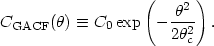
(25)

This "theory" is then convolved with the observing strategy and the predictions compared to the data. Usually limits or best-fit values are quoted on C₀ for a range of _c. In the language of the multipole moment expansion, the assumption of a GACF is equivalent to assuming

(26)

Note that this is very different from CDM, where ( + 1)C has a Sachs-Wolfe plateau followed by Doppler/adiabatic peaks.

Commonly a plot of C₀ vs _c is used to describe the sensitivity of a particular experiment to fluctuations on various scales, under the assumption that the sky correlation function is really a GACF. The GACF approximation is a simple way to understand the sensitivity of an experiment. By varying _c, one can match the "power spectrum" to the window function of the experiment (especially multi-beam experiments where the GACF power spectrum and the window function have similar shapes, which we will call "Gaussian"). The experiment is most sensitive to a GACF whose peak ( + 1)C occurs at essentially the same place as the peak of its window function W. The amplitude of fluctuations to which one is sensitive (or the "area" under the window function) is then parameterized by the minimum C₀.

For experiments in which the window function is similar to the GACF power spectrum, the approximation made in fitting with a GACf is numerically quite good. This is because, unless the underlying power spectrum varies rapidly on scales probed by the experiment, once the power spectrum is convolved with the window function, it has a "Gaussian" shape. The GACf retains its "Gaussian" shape when convolved with a Gaussian window function. Hence the two convolved spectra will look very similar (Bunn et al 1994b).

An analysis using a GACF will (roughly) take into account the peak and are of the window function of the experiment. The minimal values of C₀^1/2 will therefore be more comparable between experiments than the measured rms temperature fluctuations (which could be defined in an observer-dependent way). The correlations between nearby points will also be approximately correct for experiments with "Gaussian" window functions (and in which the window function approach is applicable; see Section 4.2). Although for some experiments, the GACf approximation may be used to give a fit to the data, the GACF assumption should be viewed with caution. One should bear in mind that the quoted C₀^1/2 is the best fit amplitude of fluctuations for a power spectrum that is a GACF with some fixed correlation angle _c. There is also little meaning in the values of C₀^1/2 at any point other than the minimum of the likelihood curve.