Annu. Rev. Astron. Astrophys. 1994. 32: 319-70 Copyright © 1994 by . All rights reserved

4.2. Window Functions

It has become conventional to describe the details of the instrument and the observing strategy in terms of a window function W which describes the sensitivity of the experiment to the modes of the spherical harmonic decomposition of the CMB temperature fluctuations. The signal seen by any experiment can then be considered as the convolution of the sky power and the window function

(27)

If one takes an ensemble average (over universes) of this expression, then a² <a²> = (2 + 1)C. Often this ensemble average is assumed when the window function is computed.

The simplest and most common window function is that due to finite beam resolution. As expected, finite resolution introduces a high- cutoff. If the beam has a Gaussian response with a Gaussian width of , the window function is (see e.g. Silk & Wilson 1980, Bond & Efstathiou 1984, White 1992)

(28)

For an experiment that measures temperatures by differencing 2- or 3-beam setups, the window functions, in addition to the beam smoothing factor, are (see e.g. Bond & Efstathiou 1987)

(29)

where is the angle between the beams. Note that these types of experiments are not sensitive to the low- modes of the multipole expansion because of the differencing. Since the high- cutoff is controlled by the beam width while the separation (or chop) controls the low- behavior, one can increase both the width and height of the window function by separating these scales as much as possible.

Such a double- or triple-beam differencing strategy is often called a square wave chop. There are, however, other scan strategies that have been used. Several experiments (in particular South Pole, Saskatoon, and MAX) use a sine wave chop, moving the beam continuously back and forth across the sky, sinusoidally in time. Additionally, the temperature is weighted by ± 1 or by a harmonic of the chop frequency. The resulting time-integrated, weighted temperature is then the "difference" assigned to that point on the sky. Window functions for these experiments can be found in Bond et al (1991b), Dodelson & Jubas (1993), White et al (1993), and Bunn et a1 (1994b). [The window function for MAX, given in White et al (1993), should be multiplied by 1.13 to account for the finite size of the beam on the calibration: see Srednicki et al (1993).] There are also several interferometer experiments which make maps of the intensity of the radiation on small patches of the sky [e.g. ATCA (Subrahmanyan et al 1993), VLA (Fomalont et al 1993), and Timbie & Wilkinson (1990)]. The window function for these experiments can be measured as the Fourier transform of the beam pattern and for accuracy needs to be supplied by the experimenters.

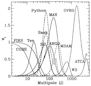
We show the window functions vs for several experiments in Figure 5. Some numbers describing the functions shown here are given in Table 2. Note that the relative heights can have as much to do with the treatment of the data as with the sensitivity, i.e. the window function that is convolved with theory should be consistent with the observers' T / T. It is worth giving an example to illustrate this. Consider a triple-beam set-up, which consists of the difference of a difference of two temperatures. The experimenters could choose to assign a measurement of T₁ - 1/2(T₂ + T₃) to a point in direction "1," or they could have chosen to take 2T₁ - (T₂ + T₃).

Figure 5. The window functions for large- and medium-scale experiments as a function of multipole. From left to right the experiments are COBE (with 10° smoothing), FIRS, Tenerife, SP91, Saskatoon (dashed), Python (dot-dashed), ARGO, MAX, MSAM (3-beam, dashed). White Dish (Method II, neglecting binning), OVRO, and ATCA, Some parameters of the window functions are displayed in Table 2.

Table 2. Parameters for the window functions ^a

Experiment	0	1	2	Max
COBE	-	-	11	1.0
FIRS	-	-	30	1.0
Ten	20	13	30	1.0
SP91	66	32	109	0.9
Sask	71	44	102	1.2
Pyth	73	50	107	1.9
ARGO	107	53	180	0.9
MAX	158	78	263	1.7
MSAM2	143	69	234	2.1
MSAM3	249	152	362	0.9
a represents the multipole at the maximum; 1 and 2 are the "half peak" points. The maximum value of the window function is also given. For MSAM we present results in 2-beam and 3-beam modes.

Common approximate formulae for the window functions or analysis procedures assume a square wave chop (e.g. Górski 1993, Gundersen et al 1993). This approximation usually does not reproduce the beam pattern on the sky all that well, although it works better for the window function. Even so, such approximation; differ from the exact results, e.g. for MAX the difference between the exact result and (29) is ~ 10% near the peak, and larger off-peak.

Given both a theory and the window function, it is straightforward to compute the expected rms temperature fluctuation. In Table 3, we show the predicted T / T_rms for various experiments, normalized to A = 1. The predictions assume full sky coverage and an "average universe," though actual experiments may measure different values due to incomplete sky coverage or cosmic variance (to be discussed later).

It is sometimes possible to define window functions that correspond to off-diagonal elements of the correlation matrix or averages of the form

(30)

which are required when fitting data. (Note that this is different from the sky-averaged correlation function of the COBE group. It is not an average over our observed sky, but the covariance matrix required when computing likelihood functions, assuming Gaussian statistics for the temperature fluctuations.) In general, the window function approach works well for computing T / T_rms or for experiments in which the data span only one dimension (such as the individual linear scans of the ACME South Pole experiment). In other cases, however, the data are two-dimensional on the sky and there can be strong anisotropies in the theoretical covariance matrix which are difficult to include in this manner. Alternative approaches are then preferable (see e.g. Srednicki et al 1993). Also, if the scanning strategy or data analysis procedure is sufficiently tortuous, the window function approach is extremely complicated and simulations of the scanning, binning, and analysis become necessary. Coarse binning of data in an experiment which scans smoothly (rather than "stepping") across the sky is one example of this, where correlations introduced by the binning will be important.

Table 3. Predictions for CMB experiments in a CDM-dominated universe ^a

	B
Experiment	0.00	0.01	0.03	0.06	0.10
COBE	2.57	2.62	2.63	2.63	2.64
FIRS	3.23	3.38	3.41	3.44	3.47
Ten	1.92	2.10	2.14	2.18	2.20
SP91	2.24	2.84	3.00	3.22	3.38
Sask	2.15	2.81	2.98	3.24	3.40
Pyth	2.69	3.84	4.10	4.49	4.76
ARGO	2.20	3.27	3.49	3.84	4.09
MAX	3.08	5.15	5.49	6.09	6.49
MSAM2	3.46	5.64	6.02	6.65	7.06
MSAM3	1.88	3.49	3.69	4.09	4.32
a We show the predicted T / Trms for various experiments, normalized to A = 1. The predictions are for an all-sky average and an "average universe"; individual experiments may measure different values due to incomplete sky coverage or cosmic variance. For MSAM the predictions are shown for 2-beam and 3-beam modes. The column B = 0 refers to an n = 1 power spectrum. All values assume CDM with 0 = 1 and h = 0.5.