APPENDIX C: PROPERTIES OF STATISTIC ²

In Section 5, we introduced the statistic ² (eq. [26]) as a measure of the coherence of the residual field between the IRAS and TF data. Here we demonstrate that it has approximately the properties of a true ² statistic, and indicate how and why it departs from true ² behavior.

The measure of residual coherence at separation is

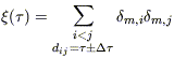
(C1)

where d_ij is the separation in IRAS-distance space between objects i and j, and _m is the normalized magnitude residual (eq. [23]). The sum runs over the N_p() distinct pairs of objects with separation ± ; note that a given object may appear in more than one of these pairs. The hypothesis we wish to test is that the IRAS-TF residuals are incoherent, which signifies a good fit on all scales. A formal statement of this condition is that the individual _m,i are independent random variables. Furthermore, the _m have been constructed to have mean zero and unit variance. Thus, our hypothesis of uncorrelated residuals implies that the expectation value of the product _{m,i m,j} vanishes for i j, and that the expectation value of its square is unity.

It follows that

(C2)

The variance of () is

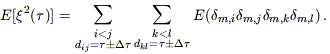
(C3)

Now the expectation value within the sum will vanish under our assumption of uncorrelated residuals unless i = k and j = l. (Notice that we cannot have i = l and j = k because of the ordered nature of the summation.) Thus, the only nonzero terms in equation (C3) are identical pairs, and it follows that E[²()] = N_p().

Because () is the sum of N_p() random variables, each of zero mean and unit variance, we are tempted to suppose that, by the central limit theorem, its distribution is Gaussian with mean zero and variance N_p() when N_p() is large. Indeed, for the 200 km s^-1 bins used in its construction (cf. Section 5.2), N_p is typically 10⁴. And, as shown in the previous paragraph, () does indeed have mean zero and variance N_p(). One also may ask about the correlation among the () for different . Specifically, one may compute

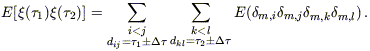
(C4)

Now it is possible to have i = k within this sum. However, because _{1 2}, if i = k then j l. Similarly, one may have j = l, but in that case i k. Thus, all of the individual expectation values in the sum vanish, and we find E[(₁) (₂)] = 0. To the extent the above considerations hold, the (_i) are independent Gaussian random variables of variance N_p(_i). It then follows that the statistic ² is distributed like a ² variable with M degrees of freedom. This is the statistic proposed in the main text as a measure of goodness of fit.

However, the central limit theorem applies only to sums of independent random variables. The individual products _{m,i m,j} that enter into () are uncorrelated in the specific sense E(_{m,i m,j}) E(_{m,k m,l}) = ^K_i,k ^K_j,l (where ^K is the Kronecker-delta symbol). However, they are not strictly independent from one another. This is because the same object can occur in more than one pair at a given . We thus expect the central limit to apply only approximately, and as a result the () are not strictly Gaussian. As a result, ² cannot be a true ² statistic.

Furthermore, just as a single object appears in many pairs at a given , it can appear in pairs at different as well. Let us suppose object i contributes to both (₁) and (₂). Then the latter are not strictly independent, even though the expectation value of their product vanishes, as shown above. This factor, too, will result in a departure from ² behavior.