Copyright © 1998 by Annual Reviews. All rights reserved
| Annu. Rev. Astron. Astrophys. 1998. 36:
599-654 Copyright © 1998 by Annual Reviews. All rights reserved |


Cosmological simulations incorporate a range of physics: gravitation, gas dynamics (adiabatic or with radiative cooling and heating), chemistry, and radiative transfer. The first is obligatory and the rest are important, even necessary, refinements. These computations are nearly always performed using comoving spatial coordinates and periodic boundary conditions so that a finite, expanding volume is embedded in an appropriately perturbed background spacetime.
2.1. Gravity Calculation and Dark Matter Evolution
Dark matter is represented in cosmological simulations by particles sampling the phase space distribution. Particles are evolved forward in time using Newton's laws written in comoving coordinates (Peebles 1980):
 |
(1) |
Here a(t) is the cosmic expansion factor (related to
redshift z by
a-1 = 1 + z), H = d ln
a / dt is the Hubble parameter,
 is the
peculiar velocity,
is the
peculiar velocity,
 is the mass density,
 is the
spatial mean density, and
is the
spatial mean density, and
 =
=
 /
/
 is the gradient
in comoving coordinates. Note that the first pair of relationships in
Equation 1 is to be integrated for every dark matter particle by using
the gravity field produced by all matter (dark and baryonic) contributing
to .
is the gradient
in comoving coordinates. Note that the first pair of relationships in
Equation 1 is to be integrated for every dark matter particle by using
the gravity field produced by all matter (dark and baryonic) contributing
to .
The time integration of particle trajectories is generally performed using a second-order accurate leapfrog integration scheme requiring only one force evaluation per timestep (Efstathiou et al 1985). While higher-order schemes would provide more accurate trajectories with longer timesteps, they are rarely used in cosmological simulations because of the costly requirement for calculating and storing additional forces or their derivatives. Mass resolution is generally considered more important than attempting to accurately follow individual particle trajectories, especially because the latter are chaotic (Goodman et al 1993 and references therein). The simulator aims to follow accurately the motions of gravitationally bound concentrations of hundreds or more particles while bearing in mind that the particles themselves are samples of the dark matter phase space.
In practice, it is preferable to use
s =  a-2 dt as the time variable
for cosmological N-body integrations instead of proper time
because the equations of motion then simplify to d2
/
ds2 = a
a-2 dt as the time variable
for cosmological N-body integrations instead of proper time
because the equations of motion then simplify to d2
/
ds2 = a
 ,
which allows a
symplectic (phase space-volume preserving) integrator for
and
d / ds
(Quinn et al 1997).
The simple
leapfrog integrator is symplectic when used with an appropriately chosen
timestep for these variables
(Hut et al 1995).
Another consideration is the use of individual timesteps
(Hernquist & Katz
1989), which can
significantly speed up highly clustered simulations if the force
evaluation is not dominated by fixed costs that are independent of
particle number.
,
which allows a
symplectic (phase space-volume preserving) integrator for
and
d / ds
(Quinn et al 1997).
The simple
leapfrog integrator is symplectic when used with an appropriately chosen
timestep for these variables
(Hut et al 1995).
Another consideration is the use of individual timesteps
(Hernquist & Katz
1989), which can
significantly speed up highly clustered simulations if the force
evaluation is not dominated by fixed costs that are independent of
particle number.
The art of N-body simulation lies chiefly in the computational algorithm used to obtain the gravitational force. The desired pair force is a softened inverse square law representing the force between two finite-size particles in order to prevent the formation of unphysical tight binaries. Evaluating the forces by direct summation over all particle pairs is prohibitive even with the largest parallel supercomputers. For N = 107, a typical number for present-day cosmological simulations, a single force evaluation by direct summation would take several hours on a 100-GFlops (1 GFlops = 109 floating point operations per second) machine but only a few seconds by fast algorithms. For collisional N-body systems like globular clusters, where greater accuracy is required, special-purpose processors like the GRAPE series (Makino et al 1997 and references therein) hold great promise. Recently a GRAPE-4 running at a sustained speed of 406 Gflops was used to simulate the formation of a single dark matter halo with high precision (Fukushige & Makino 1997). Even in large-scale cosmological simulations, when the force evaluation is separated into long-range and short-range parts, the GRAPE processor can be used effectively to speed up the computation of dense regions (Brieu et al 1995, Steinmetz 1996).
2.1.1. BARNES-HUT TREE ALGORITHM
The hierarchical tree algorithm
(Appel 1985,
Barnes & Hut 1986)
divides space recursively into a hierarchy of cells, each containing
one or more particles. If a cell of size s and distance d
(from the point where
is
to be computed) satisfies s / d <
 , the
particles in this cell are treated as one pseudoparticle located at the
center of mass of the cell. Computation is saved by replacing the
set of particles by a low-order multipole expansion due to the
distribution of mass in the cell.
, the
particles in this cell are treated as one pseudoparticle located at the
center of mass of the cell. Computation is saved by replacing the
set of particles by a low-order multipole expansion due to the
distribution of mass in the cell.
The tree algorithm has a number of important advantages
(Hernquist 1987,
1988,
Barnes & Hut 1989,
Jernigan & Porter
1989). Foremost is its
speed: O (N log N) operations are required to
compute all forces on N
particles. Force errors can be bounded and made small by choosing
< 1 and including
quadrupole and high-order moments to the
inverse square law. It is also relatively easy to implement, and
Barnes & Hut (1989)
made their code publicly
available, leading to its widespread use. Finally, the algorithm is fully
spatially adaptive - the hierarchical tree automatically refines
resolution where needed. One drawback is the relatively large amount of
memory required, from 20N to 30N words for N particles
(Hernquist 1987).
Another complication is that the tree algorithm, like direct summation
itself, does not provide periodic boundary conditions. However, this can be
corrected using a procedure known as
Ewald (1921) summation,
leading to a practical tree code for cosmological applications
(Bouchet & Hernquist
1988,
Hernquist et al 1991).
Several groups have parallelized the tree algorithm (Hillis & Barnes 1987, Makino & Hut 1989, Olson & Dorbrand 1994, Salmon & Warren 1994, Dubinski 1996, Governato et al 1997), enabling cosmological large-scale structure simulations to be performed with more than 16 million particles (Zurek et al 1994, Brainerd et al 1996).
2.1.2. PARTICLE-MESH ALGORITHM The particle-mesh (PM) method is based on representing the gravitational potential on a Cartesian grid (with a total of Ng grid points), used in solving Poisson's equation on this grid. The development of the Fast Fourier Transform (FFT) algorithm (Cooley & Tukey 1965) made possible a fast Poisson solver requiring O(Ng log Ng) operations (Miller & Prendergast 1968, Hohl & Hockney 1969, Miller 1970). Periodic boundary conditions are automatic, making this algorithm natural for cosmology, and its simplicity has led to many independent implementations (in two dimensions by Doroshkevich et al 1980, Melott 1983, Bouchet et al 1985, and subsequently in three dimensions by Centrella & Melott 1983, Klypin & Shandarin 1983, Miller 1983, White et al 1983, Bouchet & Kandrup 1985, and many others since). Hockney & Eastwood (1988) have written an excellent monograph on the PM and particle-particle/particle-mesh (P3M) methods (the latter is discussed in Section 2.1.3 below).
The PM algorithm has three steps. The mass density field is first computed on a grid. Poisson's equation is then solved for the gravity field (or the potential, which is then differenced to give the gravity field). Finally, the gravity field on the grid is interpolated back to the particles.
The first step is called mass assignment:
(, t) is
computed
on the grid from discrete particle positions and masses. The simplest
method assigns each particle to the nearest grid point (NGP), with no
contribution of mass to any other grid point.
Unsurprisingly, this method produces rather large truncation errors
(Efstathiou et al 1985,
Hockney & Eastwood
1988). The most commonly
used assignment scheme is Cloud-in-Cell (CIC), which uses multilinear
interpolation to the eight grid points defining the cubical mesh cell
containing the particle. This procedure effectively treats each
particle as a uniform-density cubical cloud. The sharp edges introduce
force fluctuations, which can be reduced by using a higher-order
interpolation scheme (e.g. Triangular Shaped Cloud or TSC, which uses
the nearest 27 grid points). These discretization errors are similar
to aliasing errors that occur in image processing. They may be reduced
further using a suitable anti-aliasing filter ("Quiet PM" of
Hockney & Eastwood
1988; see also
Ferrell & Bertschinger
1994).
The heart of the PM algorithm is the Fourier space solution of the Poisson equation for the gravitational potential:
 |
(2) |
Here  and
and  are the discrete Fourier transforms
of the mass density and potential, respectively. One may replace
the inverse Laplacian operator -1/k2 by another
multiplicative factor in Fourier space, optionally including an
anti-aliasing filter. The gravity field is then obtained by transforming
the potential back to the spatial domain and approximating the gradient
by finite differences, or by multiplication by
i
are the discrete Fourier transforms
of the mass density and potential, respectively. One may replace
the inverse Laplacian operator -1/k2 by another
multiplicative factor in Fourier space, optionally including an
anti-aliasing filter. The gravity field is then obtained by transforming
the potential back to the spatial domain and approximating the gradient
by finite differences, or by multiplication by
i  in the
Fourier
domain (with care taken when any wave vector component reaches the Nyquist
frequency). The latter method requires twice as many FFTs but leads to
slightly more accurate forces
(Ferrell & Bertschinger
1994).
in the
Fourier
domain (with care taken when any wave vector component reaches the Nyquist
frequency). The latter method requires twice as many FFTs but leads to
slightly more accurate forces
(Ferrell & Bertschinger
1994).
The third step is to interpolate the gravity from the grid back to the particles. The same interpolation scheme should be used here as in the first step (mass assignment) to ensure that self-forces on particles vanish (Hockney & Eastwood 1988).
The PM method has the advantage of speed, requiring O(N) + O(Ng log Ng) operations to evaluate the forces on all particles. For typical grid sizes (with twice as many grid points as particles in each dimension), it requires less memory and is faster per timestep than the tree algorithm. However, the forces approximate the inverse square law poorly for pair separations less than several grid spacings. Each particle has an effective diameter of about two grid spacings and a nonspherical shape (particle isotropy can be improved with an anti-aliasing filter at the expense of a larger particle diameter). Also, obtaining isolated instead of periodic boundary conditions (desirable for simulations of galaxies and galaxy groups, if not for cosmology) requires a factor of 8 increase in storage in three dimensions (Hohl & Hockney 1969), unless the complicated method of James (1977) is implemented. For high-resolution studies of galaxy dynamics, the tree code is generally considered much superior. PM codes are widely used for large-scale cosmological simulations. The PM algorithm has been parallelized by Ferrell & Bertschinger (1994).
2.1.3. P3M AND ADAPTIVE P3M The primary drawback of the particle-mesh method is that its force resolution (effectively, the particle size) is limited by the spatial grid. This limitation can be removed by supplementing the forces with a direct sum over pairs separated by less than two or three grid spacings, resulting in the particle-particle/particle-mesh (P3M) algorithm. This hybrid algorithm, first developed for plasma physics by Hockney et al (1974), was applied in cosmology by Efstathiou & Eastwood (1981). It is described in detail by Hockney & Eastwood (1988), Efstathiou et al (1985), and it was used extensively by the latter authors in a series of articles beginning with Davis et al (1985). Cosmological P3M codes have also been developed by Bertschinger & Gelb (1991), Martel (1991), and others.
The P3M method readily achieves high accuracy forces through the combination of mesh-based and direct summation forces. The mesh may be regarded as simply a convenience for providing periodic boundary conditions and removing much of the burden of computation from the direct pair summation. However, when clustering becomes strong, as occurs inevitably on small scales in realistic, high-resolution cosmological simulations, the cost of the direct summation dominates, severely degrading the performance of P3M. One solution is to replace the direct summation by a tree code (Xu 1995) or fast hardware (Brieu et al 1995, Fukushige et al 1996).
In his mesh-refined P3M algorithm, Couchman (1991) presented an elegant solution to the bottleneck of strong clustering. Subgrids are placed over regions of high density to shift some of the burden of force evaluation away from pair summation and over to a subgrid PM calculation with isolated boundary conditions. Pair summation is still done, but only for pairs whose separation is less than two to three spacings of the subgrid mesh, resulting in a substantial reduction. Multiple levels of grid refinement may be used to further reduce pair summation in dense regions. The philosophy of this method is to compute the exact desired pair force, to within a fraction of a percent accuracy for (almost) every pair, by using the combination of mesh-based PM and pair summation that gives the optimal performance. Because the pair summation no longer dominates as it does in P3M, the force computation of this new, adaptive P3M scales as O(N log N), similar to a tree code but with a somewhat smaller coefficient (Bertschinger & Gelb 1991, Couchman 1991). An example of the refinement grids used for a strongly clustered simulation is shown in Figure 1.
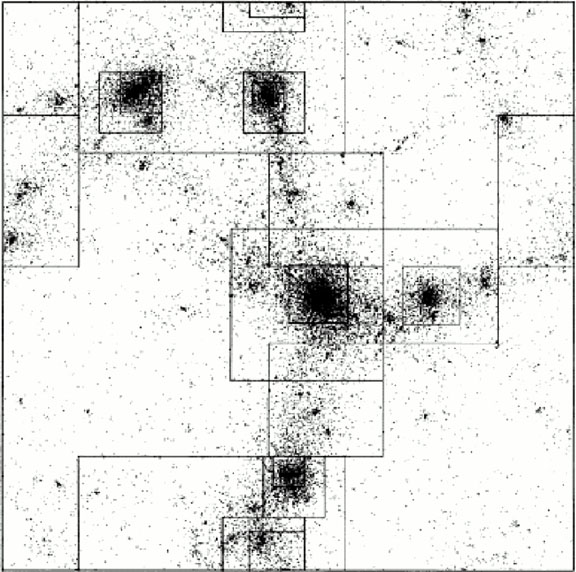 |
Figure 1. Distribution of grid refinements placed by an adaptive particle-particle/particle-mesh-smooth-particle hydrodynamics (P3M-SPH) code for the final timestep of a cluster simulation. Gas particles are shown. From Couchman et al (1995). |
The P3M algorithm has been parallelized by Ferrell & Bertschinger (1994, 1995), by Theuns (1994), and, including adaptive refinement, by Pearce & Couchman (1997) as part of their HYDRA code, which also includes smooth-particle hydrodynamics. At the present time, parallel adaptive P3M appears to be the method of choice for large cosmological N-body simulations.
2.1.4. MULTIRESOLUTION MESH METHODS Adaptive P3M avoids the resolution limit imposed by a mesh by using a combination of finer meshes and pair summation. An alternative is to dispense with pair summation altogether, instead refining or concentrating the mesh where dictated by the needs of accuracy or speed. This may be done by placing one or more levels of mesh refinement where desired and solving the Poisson equation on multiple grids. Multiple resolution algorithms have long been used in computational fluid dynamics, but only recently have they been applied in cosmology. Here the programmer must decide whether to refine only the force resolution (similar to using a finer mesh in a PM simulation) or also to refine the mass resolution (equivalent to using more particles in selected regions).
Methods that refine force but not mass resolution are similar in spirit to adaptive P3M in that they use a fixed set of (usually but not necessarily equal-mass) particles. Several groups have developed codes that automatically refine the spatial resolution where needed during the computation by using higher-resolution meshes (adaptive mesh refinement): Jessop et al (1994), Suisalu & Saar (1995), Gelato et al (1997), Kravtsov et al (1997). Unlike P3M, these codes have a variable spatial resolution of the forces. Although this leads to an effective particle size that changes as particles move across refinements, it may be closer to the spirit of phase space sampling with a resolution that might, for example, scale with the local mean particle spacing.
Another class of methods refines both the mass and force resolution by splitting particles into several lower-mass particles and using multiple grids for the force computation. All of these algorithms published to date are nonadaptive; they work with nested grids that are fixed in space. The first implementation was the hierarchical PM solver of Villumsen (1989). In Villumsen's method, an ordinary PM simulation is performed first to identify regions needing higher resolution. The simulation is then repeated with high-resolution meshes added. Particles that enter these regions (as judged by the first simulation) are split into several lower-mass particles. High-frequency waves are added to their initial displacements and velocities to simultaneously increase the sampling of the initial power spectrum. Anninos et al (1994), Dutta (1995) have implemented similar algorithms with some improvements; Dutta used a tree code for the high-resolution forces in place of PM. Splinter (1996) chose to split up massive particles only when they enter the refinement volume rather than at the beginning of the simulation. While this precludes refining the sampling of the initial power spectrum, it is less costly and closer to the spirit of adaptive refinement of both mass and force resolution.
Variants of the multiresolution approach include moving-mesh algorithms (Gnedin 1995, Pen 1995, Gnedin & Bertschinger 1996) in which the mesh used for computing the potential and force is allowed to deform. By contracting in regions of high particle density, the mesh can sample the gravitational field with higher resolution. Xu (1997) solved the Poisson equation on an unstructured mesh. In these codes, the irregularity of the mesh leads to force errors that are difficult to control, but their adaptivity and high dynamic range make these methods interesting for further study and development.
2.1.5. OTHER GRAVITY SOLVERS Various other methods have been proposed and used for computing gravitational forces. Several methods are based on multipole expansions (see Sellwood 1987), but those methods that pick out a preferred center are generally inappropriate for cosmology. The fast multipole method of Greengard & Rokhlin (1987) has attracted considerable attention, but the O(N) scaling of the original algorithm erodes in the presence of strong clustering. Adaptive multipole methods appear promising but so far have seen no use in cosmology.
More exotic approaches include direct integration of the collisionless Boltzmann equation (Hozumi 1997), treatment of collisionless dark matter as a pressureless fluid (Peebles 1987b, Gouda 1994), and even treating gravitating matter as a quantum fluid obeying the Schrödinger equation (Widrow & Kaiser 1993, Davies & Widrow 1997). These methods are useful in providing insight to the physics of gravitational clustering but are not meant to compete with other techniques as a method of general simulation.