Annu. Rev. Astron. Astrophys. 1997. 35: 101-136 Copyright © 1997 by Annual Reviews. All rights reserved

4.2. The Method of Normalized Distances for Field Galaxies

Assume that we have two standard candle (galaxy) classes, each having gaussian luminosity functions G(M₁, ) and G(M₂, ), hence simply shifted in M by M = M₁ - M₂. If both are sampled up to a sharp magnitude limit m_lim, it is easy to see that in the bias vs true distance modulus µ diagram, the bias of the second kind suffered by these two candles is depicted by curves of the same form but separated horizontally by constant µ = -M (see Figure 1a). The curve of the brighter candle achieves only at larger distances the bias suffered by the fainter candle already at smaller distances. In this way, simultaneous inspection of two or more standard-candle classes gives a new dimension to the problem of how to recognize a bias. Figure 1b shows another important property of the bias behavior. If one keeps the standard candle the same but increases the limiting magnitude by m_lim, the bias curve shifts to larger distances by µ = m_lim. This is the basis of what Sandage (1988b) calls the "adding of a fainter sample" test.

van den Bergh's morphological luminosity classes clearly showed this effect (Teerikorpi 1975a, b), and even gave evidence of the "plateau" discussed below. In the beginning of 1980s, extensive studies started to appear where the relation (Gouguenheim 1969, Bottinelli et al 1971, Tully & Fisher 1977) between the magnitude (both B and infrared) and maximum rotational velocity of spiral galaxies V_max was used as a distance indicator. In the following, the direct regression (M against fixed log V_max p) form of this TF relation is written as

(11)

There was at that time some uncertainty about which slope to use in distance determinations to individual galaxies - direct, inverse, or something between? Then Bottinelli et al (1986) argued that in order to control the Malmquist bias of the second kind, it is best to use the direct slope, so that the regression line is derived as M against the fixed observed value of p, without attempting to correct the slope for the observational error in p. The observed value of p devides the sample into separate standard candles analogous to Malmquist's star classes. A similar conclusion was achieved by Lynden-Bell et al (1988) in connection with the first kind of bias.

The importance of the direct relation is the fact that this particular slope allows one to generalize the mentioned example of two standard candles to a continuum of p values and in this way to recognize and investigate how the Malmquist bias of the second kind influences the distance determinations [that such a bias must exist also in the TF method was suspected by Sandage & Tammann (1984) and introduced on a theoretical basis in Teerikorpi (1984)]. If one inspects the whole sample (all p values clumped together) in the diagnostic log H vs d_kin diagram (cf Figure 1), the bias may not be very conspicuous. On the other hand, if one divides the sample into narrow ranges of p, each will contain a small number of galaxies, which makes it difficult to see the behavior of the bias for each separate standard candle within p ± 1/2dp. For these reasons, it is helpful to introduce so-called normalized distance d_n (Teerikorpi 1984, Bottinelli et al 1986), which transforms the distance axis in the log H vs d_kin diagram so that the separate p classes are shifted one over the other and the bias behavior is seen in its purity (see Figure 2 in this regard):

(12)

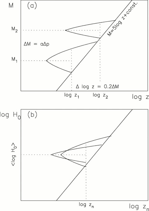Figure 2. Schematic explanation of how the method of Spaenhauer diagrams (the triple-entry correction or TEC) and the method of normalized distances (MND) are connected. Upper panel shows two Spaenhaeur (M vs log z) diagrams corresponding to TF parameters p1 and p2. The inclined line is the magnitude limit. When the data are normalized to the log H vs logzn diagram, using the TF slope a, the separate Spaenhauer diagrams "glide" one over the other and form an unbiased plateau that, among other things, can be used for determination of the Hubble constant.

In fact, one might also term this transformed distance as the effective one. This method of normalized distances (MND) uses as its starting point and test bench an approximative kinematical (relative) distance scale (d_kin, e.g. as provided by the Hubble law or Virgo-centric models) used with observed redshifts. The method usually investigates the bias as seen in the Hubble parameter log H, calculated from the (direct) TF distance for each galaxy using the (corrected) radial velocity. If the Hubble law is valid, i.e. there exists a Hubble constant H_o, then one expects an unbiased plateau at small normalized distances, a horizontal part from which the value of H_o may be estimated from the plot of the apparent H_o vs d_n. Bottinelli et al (1986) applied the method to a sample of 395 galaxies having B magnitudes and the TF parameter p and could identify clearly the plateau and determine H_o from it. Certain subtle points of the method were discussed by Bottinelli et al (1988a), who also presented answers to the criticism from de Vaucouleurs & Peters (1986), Giraud (1986). A somewhat developed version of it has recently been applied to the KLUN (kinematics of the local universe) sample constructed on the basis of the Lyon-Meudon extragalactic database and containing 5171 galaxies with isophotal diameters D₂₅ (Theureau et al 1997).