B.10.1. An Analytic Model for Einstein Rings

Most of the lensed extended sources we see are dominated by an Einstein ring - this occurs when the size of the source is comparable to the size of the astroid caustic associated with producing four-image lenses. When the Einstein ring is fairly thin, there is a simple analytic model for the formation of Einstein rings (Kochanek, Keeton & McLeod [2001]). The important point to understand is that the ring is a pattern rather than a simple combination of multiple images. Mathematically, what we identify as the ring is the peak of the surface brightness as a function of angle around the lens galaxy. We can identify the peak by finding the maximum intensity () along radial spokes in the image plane, () = ₀ + (cos, sin). At a given azimuth we find the extremum of the surface brightness of the image f_D() along each spoke, and these lie at the solutions of

(B.134)

The next step is to translate the criterion for the ring location onto the source plane. In real images, the observed image f_D() is related to the actual surface density f_I() by a convolution with the beam (PSF), f_D() = B* f_I(), but for the moment we will assume we are dealing with a true surface brightness map. Under this assumption f_D() = f_I() = f_S() because of surface brightness conservation. When we change variables, the criterion for the peak brightness becomes

(B.135)

where the inverse magnification tensor M^-1 = d / d is introduced by the variable transformation. Geometrically we must find the point where the tangent vector of the curve, M^{-1 .} d / d is perpendicular to the local gradient of the surface brightness f_S(). These steps are illustrated in Fig. B.70.

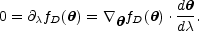
Figure B.70. An illustration of ring formation by an SIE lens. An ellipsoidal source (left gray-scale) is lensed into an Einstein ring (right gray-scale). The source plane is magnified by a factor of 2.5 relative to the image plane. The tangential caustic (astroid on left) and critical line (right) are superposed. The Einstein ring curve is found by looking for the peak brightness along radial spokes in the image plane. For example, the spoke in the illustration defines point A on the ring curve. The long line segment on the right is the projection of the spoke onto the source plane. Point A corresponds to point A' on the source plane where the projected spoke is tangential to the intensity contours of the source. The ring in the image plane projects into the four-lobed pattern on the source plane. Intensity maxima along the ring correspond to the center of the source. Intensity minima along the ring occur where the ring crosses the critical curve (e.g. point B). The corresponding points on the source plane (e.g. B') are where the astroid caustic is tangential to the intensity contours.

This result is true in general but not very useful. We next assume that the source has ellipsoidal surface brightness contours, f_S(m²), with m² = ^. S ^. where = - ₀ is the distance from the center of the source, ₀, and the matrix S is defined by the axis ratio q_s = 1 - _s 1 and position angle _s of the source. We must assume that the surface brightness declines monotonically, df_s(m²) / dm² < 0, but require no additional assumptions about the actual profile. With these assumptions the Einstein ring curve is simply the solution of

(B.136)

The ring curve traces out a four (two) lobed cloverleaf pattern when projected on the source plane if there are four (two) images of the center of the source (see Fig. B.70). These lobes touch the tangential caustic at their maximum ellipsoidal distance from the source center, and these cyclic variations in the ellipsoidal radius produce the brightness variations seen around the ring. The surface brightness along the ring is defined by f_I((), ) for a spoke at azimuth and distance () found by solving Eqn. B.135. The extrema in the surface brightness around the ring are located at the points where f_I((), ) = 0, which occurs only at extrema of the surface brightness of the source (the center of the source, = 0 in the ellipsoidal model), or when the ring crosses a critical line of the lens and the magnification tensor is singular (| M|^-1 = µ^-1 = 0) for the minima. These are general results that do not depend on the assumption of ellipsoidal symmetry.

For an SIE lens in an external shear field we can derive some simple properties of Einstein rings to lowest order in the various axis ratios. Let the SIE have critical radius b, axis ratio q_l = 1 - ₁ and put its major axis along ₁. Let the external shear have amplitude and orientation . We let the source be an ellipsoid with axis ratio q_s = 1 - _s and a major axis angle _s located at position ( cos₀, sin₀) from the lens center. The tangential critical line of the lens lies at radius

(B.137)

while the Einstein ring lies at

(B.138)

At this order, the Einstein ring is centered on the source position rather than the lens position. The orientation of the ring is generally perpendicular to that of the critical curve, although it need not be exactly so when the SIE and the shear are misaligned due to the differing coefficients of the shear and ellipticity terms in the two expressions. These results lead to a false impression that the results do not depend on the shape of the source. In making the expansion we assumed that all the terms were of the same order ( / b ~ ~ ₁ ~ _s), but we are really doing an expansion in the ellipticity of the potential of the lens e ~ e_l / 3 rather than the ellipticity of the density distribution of the lens, so second order terms in the shape of the source are as important as first order terms in the ellipticity of the potential. For example in a circular lens with no shear (₁ = 0, = 0) the ring is located at

(B.139)

which has only odd terms in its multipole expansion and converges slowly for flattened sources. In general, the ring shape is a weak function of the source shape only if the potential is nearly round and the source is almost centered on the lens. The structure of the lens potential dominates the even multipoles of the ring shape, while the structure of the source dominates the odd multipoles.

In fact, the shape of the ring can be used to simply "read off" the amplitudes of the higher order multipoles of the lens potential. This is nicely illustrated by an isothermal potential with arbitrary angular structure, = rbF() with <F()> = 1 (see Zhao & Pronk [2001], Witt et al. [2000], Kochanek et al. [2001], Evans & Witt [2001]) in the absence of any shear. The tangential critical line of the lens is

(B.140)

If and are radial and tangential unit vectors relative to the lens center and ₀ is the distance of the source from the lens center, then the Einstein ring curve is

(B.141)

with the limit showing the result for a circular source.

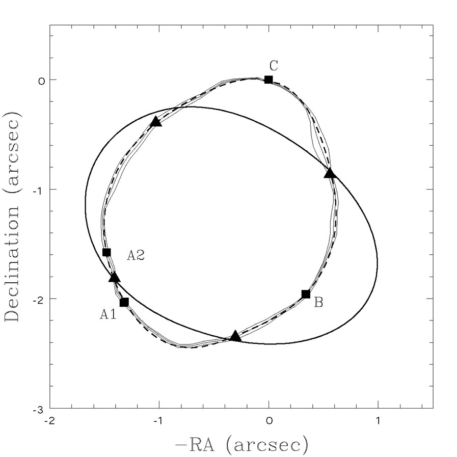
Thus, by analyzing the multipole structure of the ring curve one can deduce the multipole structure of the potential. While this has not been done non-parametrically, the ability of standard ellipsoidal models to reproduce ring curves strongly suggests that higher order multipoles cannot be significantly different from the ellipsoidal scalings. Fig. B.71 shows two examples of fits to the ring curves in PG1115+080 and B1938+666 using SIE plus external shear lens models. The major systematic problem with fitting the real data are that bright quasar images must frequently be subtracted from the image before the ring curve can be extracted, and this can lead to artifacts like the wiggle in the curve between the bright A₁ / A₂ images of PG1115+080. Other than that, the accuracy with which the ellipsoidal (plus shear) models reproduce the curves is consistent with the uncertainties. In both cases the host galaxy is relatively flat (q_s = 0.58 ± 0.02 for PG1115+080 and 0.62 ± 0.14 for B1938+666). The flatness of the host explains the "boxiness" of the PG1115+080 ring, while the B1938+666 host galaxy shape is poorly constrained because the center of the host is very close to the center of the lens galaxy so the shape of the ring is insensitive to the shape of the source. Unless the source is significantly offset from the center of the lens, as we might see for the host galaxy of an asymmetric two-image lens, it does not constrain the radial density profile of the lens very well - after considerable algebraic effort you can show that the dependence on the radial structure scales as | |⁴. It can, however, help considerably in this circumstance because it eliminates the angular degrees of freedom in the potential that make it impossible for two-image lenses to constrain the radial density profile at all.

Figure B.71. The Einstein ring curves in PG1115+080 (top) and B1938+666 (bottom). The black squares mark the lensed quasar or compact radio sources. The light black lines show the ring curve and its uncertainties. The black triangles show the intensity minima along the ring curve (but not their uncertainties). The best fit model ring curve is shown by the dashed curve, and the heavy solid curve shows the critical line of the best fit model. The model was not constrained to fit the critical line crossings.