B.10.2. Numerical Models of Extended Lensed Sources

Obviously the ring curve and its extrema are an abstraction of the real structure of the lensed source. Complete modeling of extended sources requires a real model for the surface brightness of the source. In many cases it is sufficient to simply use a parameterized model for the source, but in other cases it is not. The basic idea in any non-parametric method is that there is an optimal estimate of the source structure for any given lens model. This is most easily seen if we ignore the smearing of the image by the beam (PSF) and assume that our image is a surface brightness map. Since surface brightness is conserved by lensing, f_I() = f_S(). For any lens model with parameters p, the lens equations define the source position (, p) associated with each image position. If we had only single images of each source point, this would be useless for modeling lenses. However, in a multiply imaged region, more than one point on the image plane is mapped to the same point on the source plane. In a correct lens model, all image plane points mapped to the same source plane position should have the same surface brightness, while in an incorrect model, points with differing surface brightnesses will be mapped to the same source point. This provided the basis for the first non-parametric method, sometimes known as the "Ring Cycle" method (Kochanek et al. [1989], Wallington, Kochanek & Koo [1995]). Suppose source plane pixel j is associated with image plane pixels i = 1 ^... n_j with surface brightness f_i and uncertainties _i. The goodness of fit for this source pixel is

(B.142)

where f_s will be our estimate of the surface brightness on the source plane. For each lens model we compute ²(p) = ²_j and then optimize the lens parameters to minimize the surface brightness mismatches.

The problem with this algorithm is that we never have images that are true surface brightness maps - they are always the surface brightness map convolved with some beam (PSF). We can generalize the simple algorithm into a set of linear equations. Although the source and lens plane are two-dimensional, the description is simplified if we simply treat them as a vector f_S of source plane surface brightness and a vector f_I of image plane flux densities (i.e. including any convolution with the beam). The two images are related by a linear operator A(p) that depends on the parameters of the current lens model and the PSF. In the absence of a lens, A is simply the real-space (PSF) convolution operator. In either case, the fit statistic

(B.143)

(with uniform uncertainties here, but this is easily generalized) must first be solved to determine the optimal source structure for a given lens model and then minimized as a function of the lens model. The optimal source structure d² / d f_S = 0 leads to the equation that f_S = A^-1(p) f_I. The problem, which is the same as we discussed for non-parametric mass models in Section B.4.7, is that a sufficiently general source model when combined with a PSF will lead to a singular matrix for which A(p)^-1 is ill-defined - physically, there will be wildly oscillating source models for which it is possible to obtain ²(p) = 0.

Three approaches have been used to solve the problem. The first is LensClean (Kochanek & Narayan [1992], Ellithorpe, Kochanek & Hewitt [1996], Wucknitz [2004]), which is based on the Clean algorithm of radio astronomy. Like the normal Clean algorithm, LensClean is a non-linear method using a prior that radio sources can be decomposed into point sources for determining the structure of the source. The second is LensMEM (Wallington, Kochanek & Narayan [1996]), which is based on the Maximum Entropy Method (MEM) for image processing. The determination of the source structure is stabilized by minimizing ² + d² f_S ln(f_S / f₀) while adjusting the Lagrange multiplier such that at the minimum ² ~ N_dof where N_dof is the number of degrees of freedom in the model. Like Clean/LensClean, MEM/LensMEM is a non-linear algorithm in which solutions must be solved iteratively. Both LensClean and LensMEM can be designed to produce only positive-definite sources. The third approach is linear regularization where the source structure is stabilized by minimizing ² + f_S ^. H ^. f_S (Warren & Dye [2003], Koopmans et al. [2003]). The simplest choice for the matrix H is the identity matrix, in which case the added criterion is to minimize the sum of the squares of the source flux. More complicated choices for H will minimize the gradients or curvature of the source flux. The advantage of this scheme is that the solution is simply a linear algebra problem with (A^T(p) A(p) + H) f_S = A^T(p) f_I.

In all three of these methods there are two basic systematic issues which need to be addressed. First, all the methods have some sort of adjustable parameter - the Lagrange multiplier in LensMEM or the linear regularization methods and the stopping criterion in the LensClean method. As the lens model changes, the estimates of the parameter errors will be biased if the treatment of the multiplier or the stopping criterion varies with changes in the lens model in some poorly understood manner. Second, it is difficult to work out the accounting for the number of degrees of freedom associated with the model for the source when determining the significance of differences between lens models. Both of these problems are particularly severe when comparing models where the size of the multiply imaged region depends on the lens model. Since only multiply imaged regions supply any constraints on the model, one way to improve the goodness of fit is simply to shrink the multiply imaged region so that there are fewer constraints. Since changes in the radial mass distribution have the biggest effect on the multiply imaged region, this makes estimates of the radial mass distribution particularly sensitive to controlling these biases. It is fair to say that all these algorithms lack a completely satisfactory understanding of this problem. For radio data there are added complications arising from the nature of interferometric observations, which mean that good statistical models must work with the raw visibility data rather than the final images (see Ellithorpe et al. [1996]).

These methods, including the effects of the PSF, have been applied to determining the mass distributions in 0047-2808 (Dye & Warren [2003]), B0218+357 (Wucknitz, Biggs & Browne [2004]), MG1131+0456 (Chen, Kochanek & Hewitt [1995], and MG1654+134 (Kochanek [1995a]). We illustrate them with the Dye & Warren ([2003]) results for 0047-2808 in Fig. B.72. The mass distribution consists of the lens galaxy and a cuspy dark matter halo, where Fig. B.72 shows the final constraints on the mass-to-light ratio of the stars in the lens galaxy and the exponent of the central dark matter density cusp ( r^-). The allowed parameter region closely resembles earlier results using either statistical constraints (Fig. B.32) or stellar dynamics (Fig. B.33). In fact, the results using the stellar dynamical constraint from Koopmans & Treu ([2003]) are superposed on the constraints from the host in Fig. B.72, with the host providing a tighter constraint on the mass distribution than the central velocity dispersion. The one problem with all these models is that they have too few degrees of freedom in their mass distributions by the standards we discussed in Section B.4.6. In particular, we know that four-image lenses require both an elliptical lens and an external tidal shear in order to obtain a good fit to the data (e.g. Keeton, Kochanek & Seljak [1997]), while none of these models for the extended sources allows for multiple sources of the angular structure in the potential. In fact, the lack of an external shear probably drives the need for dark matter in the 0047-2808 models. Without dark matter, the decay of the stellar quadrupole and the low surface density at the Einstein ring means that the models generate too small a quadrupole moment to fit the data in the absence of a halo. The dark matter solves the problem both through its own ellipticity and the reduction in the necessary shear with a higher surface density near the ring (recall that 1 - <>). Again see the need for a greater focus on the angular structure of the potential.

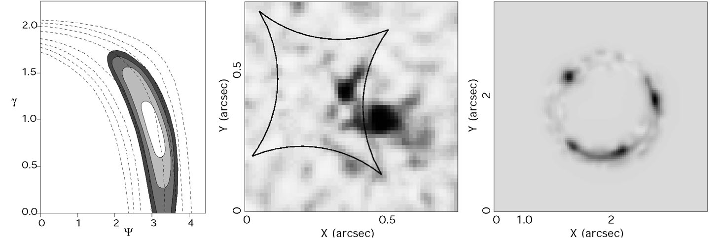Figure B.72. Models of 0047-2808 from Dye & Warren ([2003]). The right panel shows the lensed image of the quasar host galaxy after the foreground lens has been subtracted. The middle panel shows the reconstructed source and its position relative to the tangential (astroid) caustic. The left panel shows the resulting constraints on the central exponent of the dark matter halo ( r-) and the stellar mass-to-light ratio of the lens galaxy. The dashed contours show the constraints for the same model using the central velocity dispersion measurement from Koopmans & Treu ([2003]).