1. INTRODUCTION

It has long been appreciated that the CMB anisotropy could be a powerful probe of cosmology. The foundations of the anisotropy calculations we do today were set out over thirty years ago by Sachs & Wolfe (1967), Rees (1968), Silk (1968), Peebles & Yu (1970), and Sunyaev & Zeldovich (1970). Plots of the acoustic peaks were shown in Doroskevich, Zeldovich, & Sunyaev (1978) and Bond & Efstathiou (1984) gave the results of detailed numerical calculations.

On the measurement side, the tension between expectations and continuously improving upper limits (e.g., Weiss 1980, Wilkinson 1985, Partridge 1995) was finally alleviated by the discovery of the anisotropy by COBE (Smoot et al. 1992). At that time, the measured Sachs-Wolfe plateau (l < 20) was a factor of two higher than expectations based on the standard cold dark matter model in which _m 1. ⁽¹⁾ There were many measurements of the anisotropy at the COBE scales and finer between 1992 and 2000 (e.g., see Page 1997 for a table) that culminated in observations of the first acoustic peak (Dodelson & Knox 2000, Hu 2000, Pierpaoli, Scott & White 2000, Knox & Page 2000).

Amidst theories that did not survive observational tests and false clues, a standard cosmological model emerged. Even over a decade ago, the evidence from a majority of independent tests indicated _m 0.3 (e.g., Ostriker 1993). It was realized by many that a flat model (_k = 0) with a significant cosmic constituent with negative pressure, such as a cosmological constant, was a good fit to the data. Then, in 1998 measurements of type 1a supernovae (Riess et al. 1998, Perlmutter et al. 1999) directly gave strong indications that the universe was accelerating as would be expected from a cosmological constant. The state of the observations in 1999 is summarized in Figure 1. If the Einstein/Friedmann equations describe our universe, the data were telling us that the universe is spatially flat with matter density _m 0.3 and 0.7. Independent analyses came to similar conclusions (e.g., Lineweaver 1998, Tegmark & Zaldarriaga 2000). The story since the last IAU meeting is that the concordance model does in fact describe virtually all cosmological observations astonishing well. There is now a well agreed upon standard cosmological model (Spergel et al. 2003, Freedman & Turner 2003).

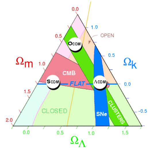Figure 1. The Cosmic Triangle from Bahcall et al. (1999). This shows the concordance model for cosmological observations at the end of the last millenium. Three different classes of observations, supernovae, clusters, and CMB anisotropy, are consistent if we live in a spatially flat universe with a cosmological constant.

In the rest of this article we briefly review the CMB observations in Section 2 and summarize what we learn from (almost) just the CMB in Section 3. We then, in Section 4, outline the things we learn by combining the CMB with other maps of the cosmos, in particular the 2dF Galaxy Redshift Survey (Colles et al. 2001). In Section 5 we indicate the sorts of things we hope to learn by using the CMB as a back light for lower redshift phenomena. We conclude in Section 6.

¹ We use the convention that _m = _cdm + _b + is the cosmic density in all matter components where cdm is cold dark matter, b is for baryons, and is for neutrinos; _r is the cosmic radiation density (now minuscule); is the corresponding density for a cosmological constant; and _k is the corresponding curvature parameter. The Friedmann equation tells us: 1 + _k + _m = _tot + _k. The physical densities are given by, for example, _b = _b h². Back.