7.4. Temporal Structure in Internal shocks

Type-II behavior arises naturally in the internal shock model. In this model different shells have different Lorentz factors. These shells collide with each other and convert some of their kinetic energy into internal energy and radiate (Fig. 18). If the emission radius is sufficiently small angular spreading will not erase the temporal variability. This requires R_E 2_E² c T. This condition is always satisfied as internal shocks take place at R_E = R_s ² with _E . Since < we have T = / c > T_ang = R_E / 2_E² c = / c = T. Clearly multiple shells are needed to account for the observed temporal structure. Each shell produces an observed peak of duration T and the whole complex of shells (whose width is ) produces a burst that lasts T = / c. The angular spreading time is comparable to the temporal variability produced by the "inner engine". They determine the observed temporal structure provided that they are longer than the cooling time.

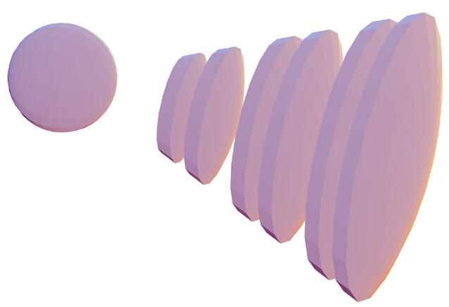Figure 18. The internal shock scenario. The source produces multiple shells as shown in this figures. The shells will have different Lorentz factors. Faster shells will catch up with slower ones and will collide, converting some of their kinetic energy to internal energy. This model is Type-II and naturally produces variable bursts. from [20].

Before concluding that internal shocks can actually produce GRBs we must address two issues. First, can internal shocks produce the observed variable structure? Second, can it be done efficiently? We will address the first question here and the second one in section 8.6 where we discuss energy conversion in internal shocks.

Mochkovitch, Maitia and Marques [32] and Kobayashi, Piran & Sari [33] used a simple model to calculate the temporal profiles produce by an internal shock. According to this model the relativistic flow that produces the shocks is characterized by multiple shells, each of width l and with a separation L. The shells are assigned random Lorentz factors (varying in the range [_min, _max]) and random density or energy. One can follow the motion of the shell and calculate the time of the binary (two-shell) collisions that take place, until all the shells that could collide have collided and the remaining flow has a monotonically decreasing velocity. The energy generated and the emitted radiation in each binary encounter are then combined to a synthetic sample of a temporal profile.

The emitted radiation from each binary collision will be observed as a single pulse characterized by an amplitude and a width. The amplitude depends on the amount of energy converted to radiation in a given collision (see 8.6). The time scale depends on the cooling time, the hydrodynamic time, and the angular spreading time. The internal energy is radiated via synchrotron emission and inverse Compton scattering. In most of cases, the electrons' cooling time is much shorter than the hydrodynamic time scale [103, 232, 18] so we consider only the latter two.

The hydrodynamic time scale is determined by the time that the shock crosses the shell, whose width is d. In fact there are two shocks: a forward shock and a reverse shock. Detailed calculations [33] reveals that this time scale (in the observer's rest frame) is of order of the light crossing time of the shell, that is: d / c.

Let the distance between the shells be . A collision takes place at / ² and the angular spreading yields an observed pulse whose width is ~ / c. If > d the overall pulse width T is determined by angular spreading. The shape of the pulse become asymmetric with a fast rise and a slower decline (Fig. 19) which GRBs typically show (see section 2.2). The amplitude of an individual pulse depends on the energy produced in the collision, which we calculate latter in section 8.6.

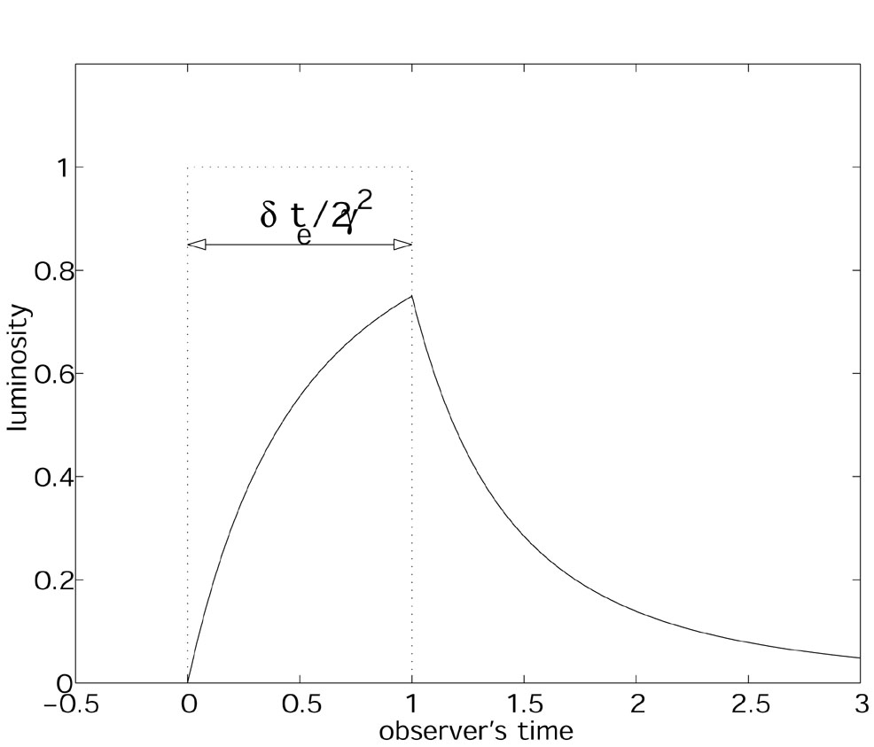Figure 19. A peak produced by a collision between two shells. The luminosity plotted versus the arrival time. The solid line corresponds to R = c te and the dotted line corresponds to R = 0, from [33]

Typical synthetic temporal profile are shown in Fig. 20. Clearly, internal shocks can produce the observed highly variable temporal profiles, provided that the source of the relativistic particles, the "inner engine", produces a sufficiently variable wind. Somewhat surprisingly the resulting temporal profile follows, to a large extent, the shape of the pulse emitted by the source. Long bursts require long relativistic winds that last hundred seconds, with a rapid variability on a time scale of a fraction of a second. Thus, unlike previous worries [78, 236] we find that there is some direct information on the "inner engine" of GRBs: It produces the observed complicated temporal structure. This severely constrains numerous models.

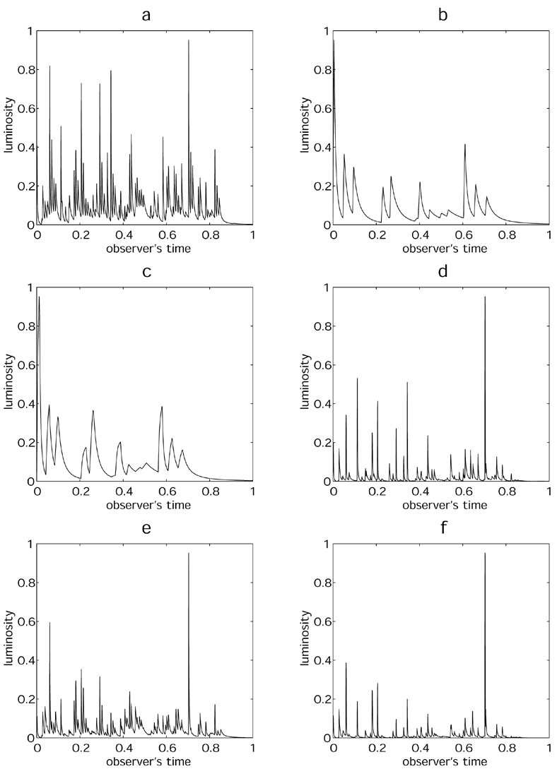Figure 20. Luminosity vs. observer time, for different synthetic models a: min = 100, max = 1000, N = 100, = - 1 and L / l = 5 b: min = 100, max = 1000, N = 100, = 1 and L / l = 5 c: min = 100, max = 1000, N = 20 , = - 1 and L / l = 5 d: min = 100, max = 1000, N = 20 , = - 1 and L / l = 1 e: min = 100, max = 1000, N = 100, random energy with Emax = 1000 and L / l = 5 f: min = 100, max = 1000, N = 100, random density with max = 1000 and L / l = 5. From [33].