9.3. Synchrotron Emission from a Relativistic Decelerating Shell

We proceed now to estimate the expected instantaneous spectrum and light curve from a relativistic decelerating shell. The task is fairly simple at this stage as all the ground rules have been set in the previous sections. We limit the discussion here to a spherical shock propagating into a homogeneous external matter. We consider two extreme limits for the hydrodynamic evolution: fully radiative and fully adiabatic. If _e is somewhat less than unity during the fast cooling phase (t < t_fs) then only a fraction of the shock energy is lost to radiation. The scalings will be intermediate between the two limits of fully radiative and fully adiabatic discussed here.

For simplicity we assume that all the observed radiation reaches the observer from the front of the shell and along the line of sight. Actually to obtain the observed spectrum we should integrate over the shell's profile and over different angles relative to the line of sight. A full calculation [259] of the integrated spectrum over a Blandford-McKee profile shows that that different radial points from which the radiation reaches the observers simultaneously conspire to have practically the same synchrotron frequency and therefore they emit the same spectrum. Hence the radial integration over a Blandford-McKee profile does not change the observed spectrum (note that this result differs from the calculation for a homogeneous shell [255]). On the other hand the contribution from angles away from the line of sight is important and it shapes the observed spectrum, the light curve and the shape of the Afterglow (see Fig 26).

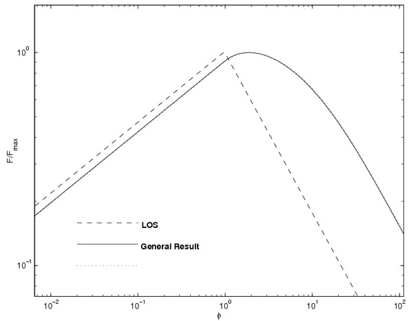Figure 26. Calculated spectra or light curve from a Blandford-McKee solution. F(t) is plotted as a function of Const. × t3/2. Thus if we consider a constant time this figure yields the spectrum while if we consider a fixed frequency it yields the light curve. The solid curve depictes emission from the full fireball. The dashed line depictes the spectrum resultsing from emission along the line of sight. From [259].

The instantaneous synchrotron spectra from a relativistic shock were described in section 8.2.4. They do not depend on the hydrodynamic evolution but rather on the instantaneous conditions at the shock front, which determines the break energies _c and _m. The only assumption made is that the shock properties are fairly constant over a time scale comparable to the observation time t.

Using the adiabatic shell conditions (Eqs. 122-123), Eqs. 44 for the shock conditions, Eq. 56 for the synchrotron energy and Eq. 62 for the "cooling energy" we find:

(132)

where t_d is the time in days, D₂₈ = D / 10²⁸ cm and we have ignored cosmological redshift effects. Fig. 22 depicts the instantaneous spectrum in this case.

For a fully radiative evolution we find:

(133)

where we have scaled the initial Lorentz factor of the ejecta by a factor of 100: _{100 0} / 100. These instantaneous spectra are also shown in Fig. 22.

9.3.1. Light Curves

The light curves at a given frequency depend on the temporal evolution of the break frequencies _m and _c and the peak power N_e P_syn(_e,min) (see Eq. 66). These depend, in turn, on how and N_e scale as a function of t.

The spectra presented in Fig. 22 show the positions of _c and _m for typical parameters. In both the adiabatic and radiative cases _c decreases more slowly with time than _m. Therefore, at sufficiently early times we have _c < _m, i.e. fast cooling. At late times we have _c > _m, i.e., slow cooling. The transition between the two occurs when _c = _m at t_fs (see Eq. 126). At t = t_fs, the spectrum changes from fast cooling (Fig. 22a) to slow cooling (Fig. 22b). In addition, if _e 1, the hydrodynamical evolution changes from radiative to adiabatic. However, if _e << 1, the evolution remains adiabatic throughout.

Once we know how the break frequencies, _c, _m, and the peak flux F_{, max} vary with time, we can calculate the light curve. Consider a fixed frequency (e.g. = 10¹⁵ ₁₅ Hz). From the first two equations in (132) and (133) we see that there are two critical times, t_c and t_m, when the break frequencies, _c and _m, cross the observed frequency :

(134)

(135)

There are only two possible orderings of the three critical times, t_c, t_m, t_fs, namely t_fs > t_m > t_c and t_fs < t_m < t_c. We define the critical frequency, ₀ = _c(t_fs) = _m(t_fs):

(136)

When > ₀, we have t_fs > t_m > t_c and we refer to the corresponding light curve as the high frequency light curve. Similarly, when < ₀, we have t_fs < t_m < t_c, and we obtain the low frequency light curve.

Fig. 27a depicts a typical high frequency light curve. At early times the electrons cool fast and < _m and < _c. Ignoring self absorption, the situation corresponds to segment B in Fig. 22, and the flux varies as F ~ F_{, max}( / _c)^1/3. If the evolution is adiabatic, F_{, max} is constant, and F ~ t^1/6. In the radiative case, F_{, max} ~ t^-3/7 and F ~ t^-1/3. The scalings in the other segments, which correspond to C, D, H in Fig. 22, can be derived in a similar fashion and are shown in Fig. 27a.

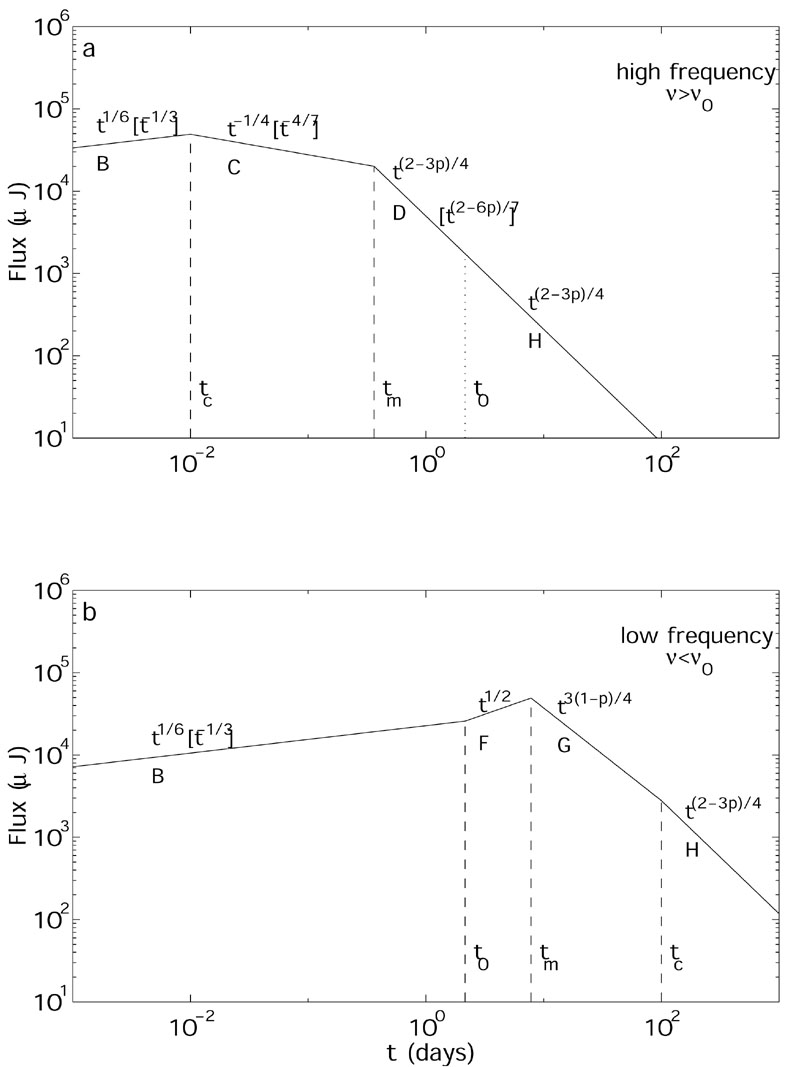Figure 27. Light curve due to synchrotron radiation from a spherical relativistic shock, ignoring the effect of self-absorption. (a) The highfrequency case ( > 0). The light curve has four segments, separated by the critical times, tc, tm, t0. The labels, B, C, D, H, indicate the correspondence with spectral segments in Fig. 22. The observed flux varies with time as indicated; the scalings within square brackets are for radiative evolution (which is restricted to t < t0) and the other scalings are for adiabatic evolution. (b) The low frequency case ( < 0). From [246].

Fig. 27b shows the low frequency light curve, corresponding to < ₀. In this case, there are four phases in the light curve, corresponding to segments B, F, G and H. The time dependences of the flux are indicated on the plot for both the adiabatic and the radiative cases.

For a relativistic electron distribution with a power distribution ^-p the uppermost spectral part behaves like ^-p/2. The corresponding temporal index (for adiabatic hydrodynamics) is -3p/4. In terms of the spectral index , this yields the relation F t^(1-3)/2. Alternatively for slow cooling there is also another frequency range (between _m and _c) for which the spectrum is given by ^-(p-1)/2 and the temporal decay is -3(p - 1) / 4. Now we have F t^-3/2. Note that in both cases there is a specific relation between the spectral index and the temporal index which could be tested by observations.

9.3.2. Parameter Fitting for GRBs from Afterglow Observation and GRB970508

Shortly after the observation of GRB970228 Mészáros et al. [22] showed that the decline in the intensity in X-ray and several visual bands (from B to K) fit the afterglow model well (see fig. 28). The previous discussion indicates that this agreement shows that the high energy tail (or late time behavior) is produced by a synchrotron emission from a power law distribution.

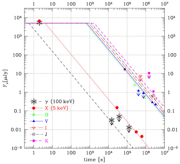Figure 28. Decline in the afterglow of GRB970228 in different wavelength and theoretical model, from [22]

There are much more data on the afterglow of GRB970508. The light curves in the different optical bands generally peak around two days. There is a rather steep rise before the peak which is followed by a long power law decay (see figs. 6, 7). In the optical band the observed power law decay for GRB970508 is -1.141 ± 0.014 [151]. This implies for an adiabatic slow cooling model (which Mészáros et al. [22] use) a spectral index = - 0.761 ± 0.009. However, the observed spectral index is = - 1.12 ± 0.04 [260]. A fast cooling model,for which the spectral index is p/2 and the temporal behavior is 3p/4 - 1/2, fits the data better as the temporal power law implies that p = 2.188 ± 0.019 while the spectral index implies, consistently, p = 2.24 ± 0.08 [246, 261] (see Fig. 29). Unfortunately, at present this fit does not tell us much about the nature of the hydrodynamical processes and the slowing down.

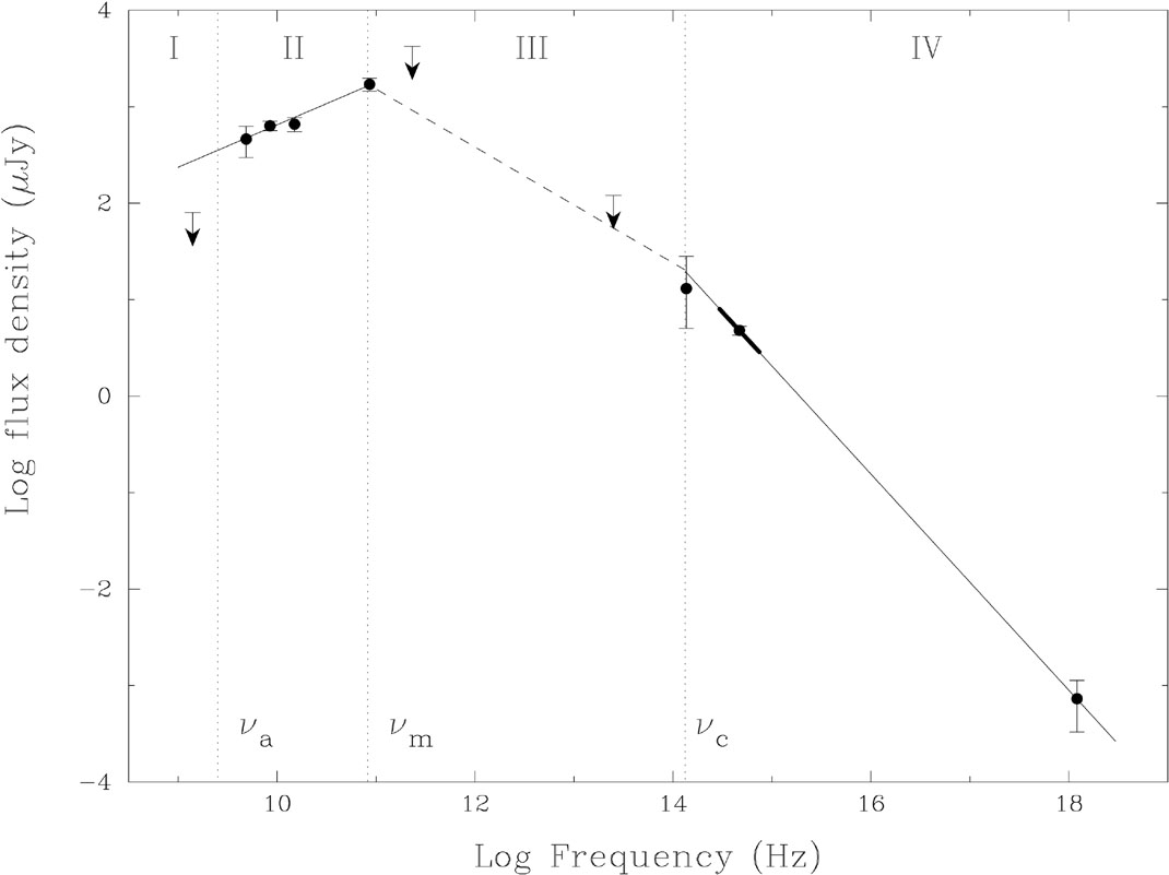Figure 29. The X-ray to radio spectrum of GRB 970508 on May 21.0 UT (12.1 days after the event). The fit to the low-frequency part, 4.86-86 GHz = 0.44 ± 0.07, is shown as well as the extrapolation from X-ray to optical (solid lines). The local optical slope (2.1-5.0 days after the event) is indicated by the thick solid line. Also indicated is the extrapolation F -0.6 (lines). Indicated are the rough estimates of the break frequencies a, m and c for May 21.0 UT from [260]

Using both the optical and the radio data on can try to fit the whole spectrum and to obtain the unknown parameters that determine the fireball evolution [248, 249]. Wijers and Galama [248] have attempted to do so using the spectrum of GRB970508. They have obtained a reasonable set of parameters. However, more detailed analysis [249] reveals that the solution is very sensitive to assumptions made on how to fit the observational data to the theoretical curve. Moreover, the initial phase of the light curve of GRB970508 does not fit any of the theoretical curves. This suggests that at least initially an additional process might be taking place. Because of the inability to obtain a good fit for this initial phase there is a large uncertainty in the parameters obtained in this way.

No deviation in the observed decaying light curve from a single power law was observed for GRB970508, until it faded below the level of the surrounding nebula. This suggests that there was no significant beaming in this case. If the outflow is in the form of a jet the temporal behavior will change drastically when the opening angle of the jet equals 1 / [258].